Lecture 7, part 4 of 4
| PLNT4610/PLNT7690
Bioinformatics Lecture 7, part 4 of 4 |
| Bayesian methods represent a
fundamental intellectual breakthrough to solving problems
in almost any field. Bayesian methods attack problems by
asking the question, "Would
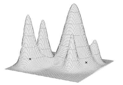
we recognize the best answer if we saw it?". If we know how to answer that question, the most straightforward solution would be to test all possible answers (trees), and see which one was the most likely one to generated the observed data. To illustrate, imagine the set of all probabilities as a surface, each point on the surface representing the probability that a given tree would generate the alignment we see. The best trees, and their variants, will appear as peaks on the surface, and the worst trees and their variants will appear as valleys. |
 from http://artedi.ebc.uu.se/course/X3-2004/Phylogeny/Phylogeny-TreeSearch/Phylogeny-Search.html |
P(model
|
data)
|
ie. what is the
probability that the model would generate the data we actually see? |
Bayes Theorem: |
where P(Model|Data)
is the posterior probability of the model, given the
data
P(Data|Model) is the probability of the data, given the model P(Model) is the prior probability of the model (without any knowledge of the data). eg, if all models are equally valid, P(model) = 1/the number of possible models P(Data) is the prior probability of the data (without any knowledge of the model) |
| prior probability
- the probability calculated on theoretical grounds,
with no knowledge of the experimental data posterior probability - the probability of seeing a particular result, calculated from the experimental data. |
|
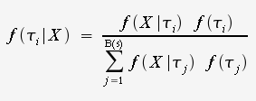
 given alignment X, the posterior probability of
the tree is
 |
numerator - one tree denominator - all trees |
 )
is the probability that tree
  would
generate alignment X
 is the set of branch lengths for a given tree
 is the set of substitution
parameters (eg. base substitution)
 ) is
the prior probability of tree
  , that
is, the probability of all of the mutational events
going from the ancestral node of the tree, to give all
of the observed nodes. This is usually nothing more than
the reciprocal of the number of all possible trees.
, that
is, the probability of all of the mutational events
going from the ancestral node of the tree, to give all
of the observed nodes. This is usually nothing more than
the reciprocal of the number of all possible trees.For
an unrooted tree with s branches, |
For
a rooted tree, |
 . We can sample the solution space.
If we take enough samples, we will find an answer that is
close to the optimal answer. The MCMC algorithm
works as follows:
. We can sample the solution space.
If we take enough samples, we will find an answer that is
close to the optimal answer. The MCMC algorithm
works as follows:| PLNT4610/PLNT7690
Bioinformatics Lecture 7, part 4 of 4 |