 Gaussian and GaussView Computation and Visualization Notes PageGaussian and GaussView Computation and Visualization Notes Page
Gaussian03W is a computational chemistry program, which can calculate energies, a variety of molecular properties, optimize molecular geometries, and predict spectroscopic properties of the system (i.e. UV-Vis, NMR, IR, EPR, Mossbauer, CD, etc.). It combines a variety of computational methods, including Density Functional Theory, Hartree-Fock as well as correlated or post-Hartree-Fock, Semi-empirical, and Molecular Mechanics approaches. In the first lab, you will learn how to do the following:
Construct an input file using GaussView
Construct an input file using Gaussian03W or text editor
Start Gaussian03W Job from GaussView or Gaussian03W
What should be in the lab report
In this lab you will make your first Gaussian03W calculation on a small transition-metal complex. You will use the graphical interface developed by Gaussian Inc. called GaussView . You also can generate an initial coordinates file using HyperChem or other available program by saving those in Brookhaven PDB, MDL, Sybyl Mol2, or CIF formats. So lets get started. Make sure you have a laboratory notebook ready to document the progress of this lab.
 Start the GaussView program by clicking on the GaussView icon from start menu. The following GaussView windows should appear:
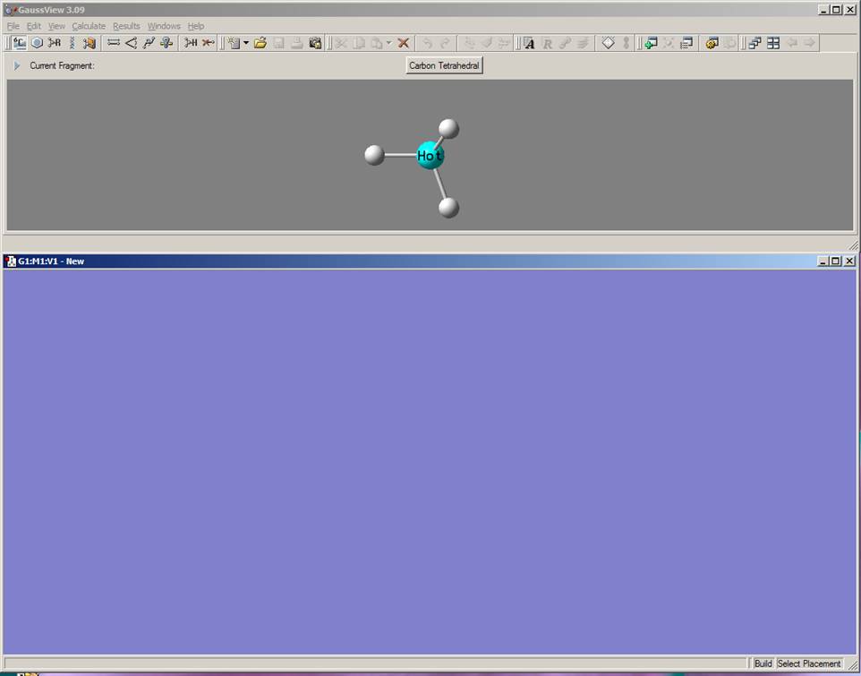
 First, you will build a simple diamagnetic transition-meal complex, [CrOCl4]2-. Click on the element fragment button on the toolbar, which is located just above the current picture in the gray window. This will open another window with the periodic table in it. Click on the chromium symbol in the periodic table. As a result, you will see the different coordination polyhedrons available for the chromium atom in GaussView at the bottom of the Periodic Table. Unfortunately, there is no way to directly choose tetragonal pyramidal coordination for the metal in GaussView yet, so choose octahedral coordination. Click on the Molgroup window (blue window with nothing in it) and the coordination polyhedron you have selected will appear there along with attached hydrogen atoms:
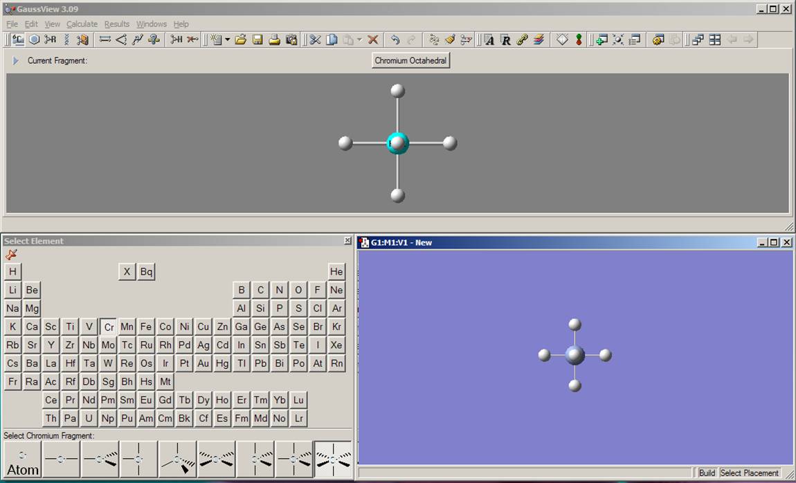
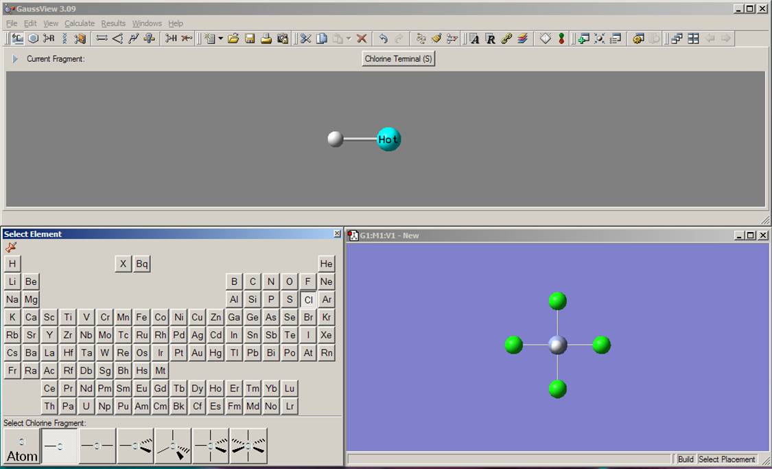 In the next step, you need to add the equatorial chlorine atoms to the chromium center (if the periodic table window disappeared, click again on the element fragment button on the toolbar). Select chlorine from the periodic table. From the possible selections at the bottom of the periodic table, choose the chlorine atom with the single bond. Clicking on the equatorial hydrogen atoms in the Molgroup window, change those to the chlorine atoms. Currently the model should look like the one presented on the picture:
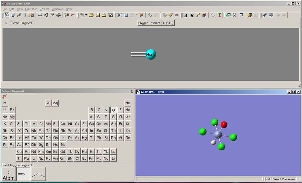 Now you need to add the axial oxygen atom to the chromium center (if the periodic table window disappeared, click again on the element fragment button on the toolbar). Select oxygen from the periodic table. From the possible selections at the bottom of the periodic table, choose the oxygen atom with the double bond. Play with the mouse and figure out how you can rotate (click the mouse and move it left or right) as well as enlarge or shrink (press the "Ctrl" key, click the mouse, and move it up or down) the molecule. Click on the axial hydrogen in the Molgroup window and change it to the oxygen atom. Currently, the model should look like the one presented on the picture:
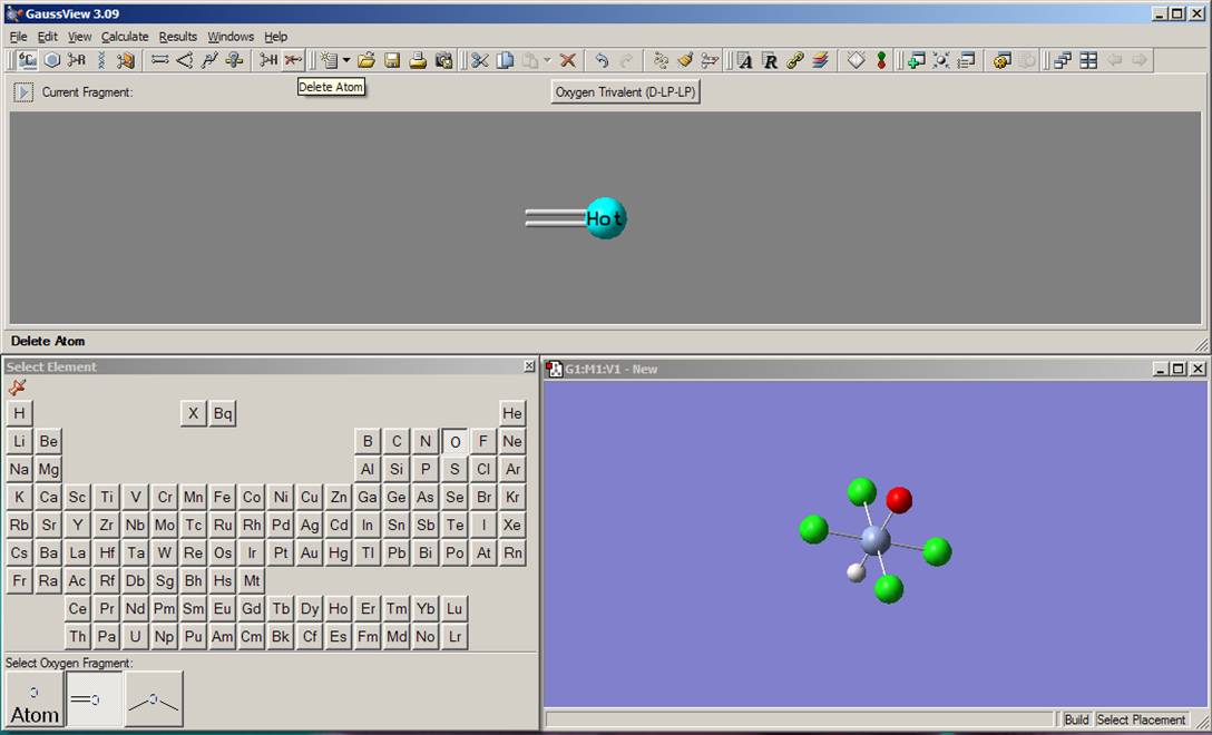
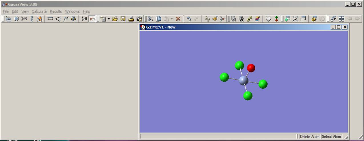 Finally, you need to delete the axial hydrogen atom lefts in the model. Select delete atom function from the toolbar menu as it shown on the left picture. Click on the axial hydrogen on the Molgroup window. Currently, the model should look like the one presented on the right picture:
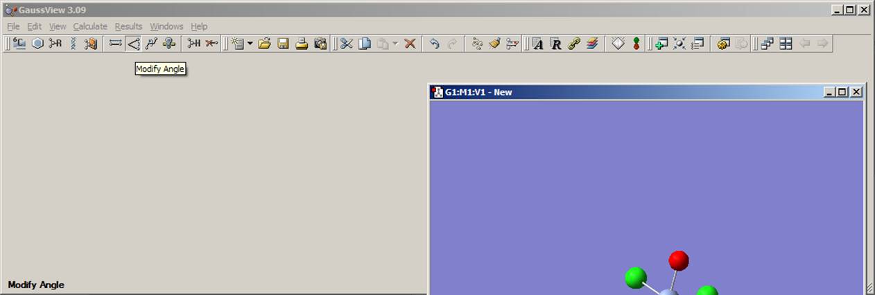
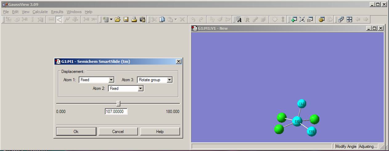 By rotating the molecule, you can easily see that the O=Cr-Cl angle is equal to 900, which is different from the real structure in which this angle should be close to 1070. Thus, in the next step, you need to change O=Cr-Cl angle. To do this, select the modify angle function from a toolbar menu as shown on the left picture above. Click on the oxygen, chromium, and then chlorine atom. As a result, the angle modification window will appear as shown on the right figure above. For the atom 1 (oxygen) and atom 2 (chromium), choose the "Fixed" command from pop-up menu and the "Rotate group" command for atom 3 (chlorine) as presented on the figure above. In the angle value window, change 90.000 on 107.0000 and click the "OK" button. Repeat this procedure for all four O=Cr-Cl angles. The current model should look like the one presented on the right picture above. Rotate the molecule to make sure that all angles were changed.
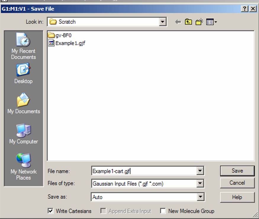 Go to the "File" menu and save the input file. Do it again, and check "Write Cartesians" box to save cartesian coordinates in a separate file. We will see the difference between our input files later in this lab.
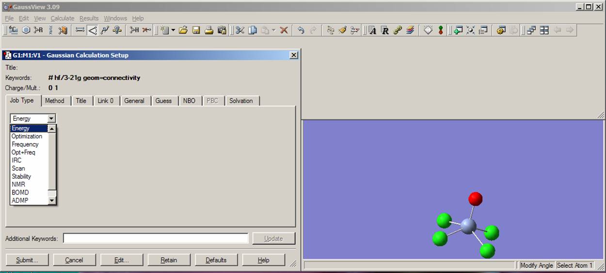 Now you are almost ready to start your calculation. You just need to tell Gaussian03W, which kind of calculation you would like to perform. In order to do this, first click on the "Calculate" menu and select the "Gaussian" command. The Gaussian Calculation Setup window will appear as presented on the figure. From the pop-up menu located in the Job type bookmark select "Energy". Next, type "pop=full" and "test" words in the "Additional Keywords" menu line. The current view should be close to that presented on the picture:
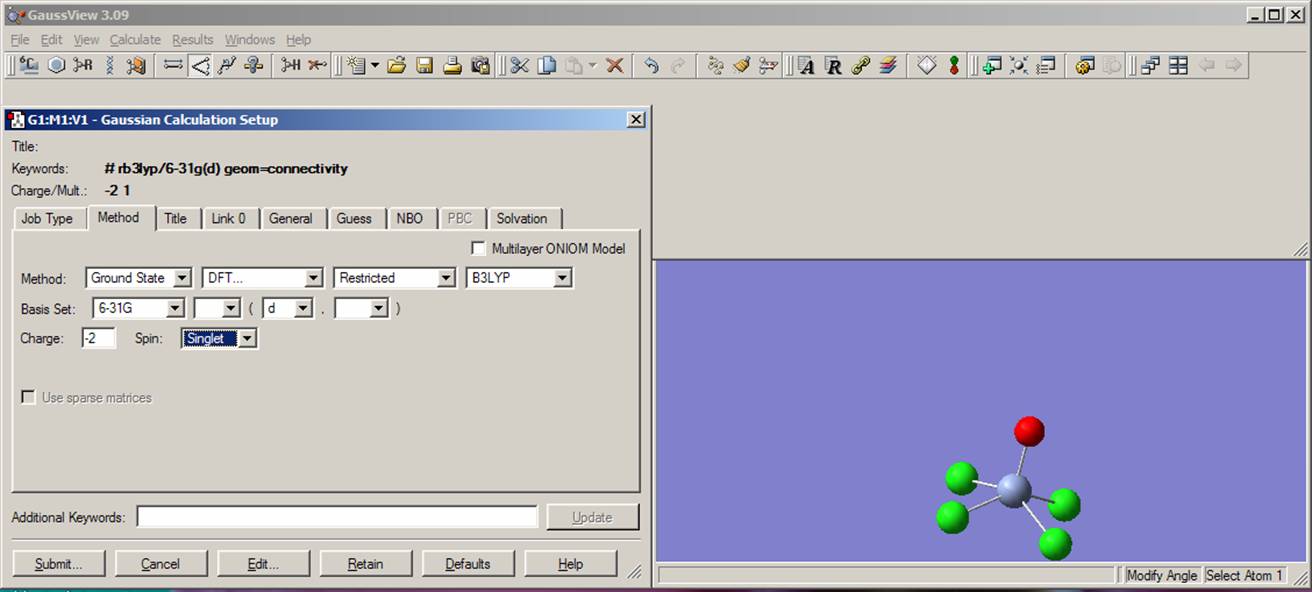 Select the following values from the next bookmark "Method": Method: "Ground State" "DFT" "Restricted", "B3LYP"; Basis Set: "6-31G" and "d"; Charge "-2"; Spin "Singlet". The current view should be close to that presented on the picture:
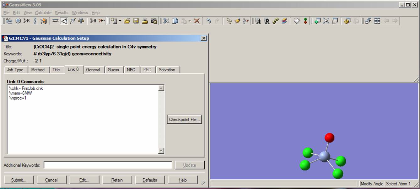 In the "Title" bookmark window type the name of the job or compound, i.e. "[CrOCl4]2- diamagnetic complex; my first job". Now move to the "Link 0" bookmark and specify the name of checkpoint file in the first line, i.e. FirstJob.chk. You will find more information on %mem and %proc commands below, when you will be constructing an input file from the beginning. The current view should be close to that presented on the picture:
Finally, check the "Additional Print" box in the "Guess" bookmark. Now you are ready to start your first calculation, but first lets find out how you can construct an input file from the beginning without using GaussView.
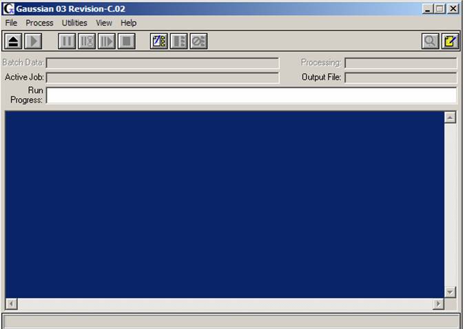 First, open the Gaussian03W program from Windows menu. Lets become a little bit more familiar with the window, which will appear (see figure on the right). In the first menu line all commands are obvious and it is always a good idea to click on the each of the menu buttons (File, Process, Utilities, View, and Help) to have a look what is located under the each one. The second line consists of job control icons and the meaning of the first six ones from the left to the right is: "Open file", "Run current job", "Pause current job", "Pause current job after next link", "Resume calculations", and "Stop current job". The fourth line ("Active Job" line) will indicate the input file name and path as well as output file name. The fifth line ("Run Progress" line) will display the current working link of the Gaussian03W program. The large Gaussian output area will allow you to monitor the current status of output information. Finally, the status line on the bottom will provide you with information on what the current Gaussian03W link is doing.
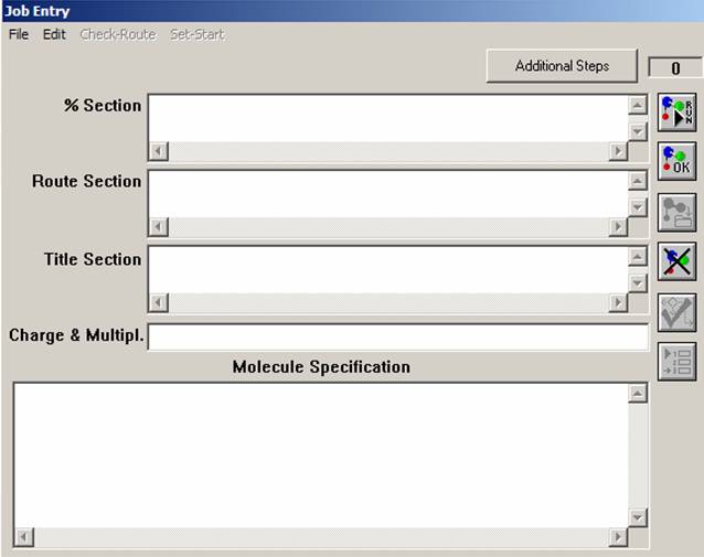 Now open the "File" menu and select "New" command. Similar to that presented on the figure, a Gaussian03W window should appear. The "%Section" specifies the path for some important files, amount of memory that will be used and the other commands mentioned below. The "Route Section" specifies the theoretical model, basis set, type of job, and which additional information will be printed into the output file. The "Title Section" briefly describes the job. The "Charge & Multipl." section defines charge and multiplicity of the molecule of interest. Finally, the "Molecular Specification" section should have atomic coordinates and some additional information, which will be discussed in the other labs.
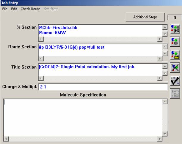 Before you start to put information into blank lines in the job entry window, just keep in mind that the Gaussian03W program can read Single-line Input (valid for "%Section" and "Charge & Multipl." line) and Multiple-line Input (valid for all other lines). The Multiple-line Input commands should be separated by a blank line. In our first job, you do not need to worry about this, but it will become important when you will be constructing the ASCII input file below. First, fill the "%Section" command line, which is an analogue of the "Link 0" bookmark in the GaussView menu. Every single line in this section starts with "%" sign. For most jobs, you will not use this line, but it is always a good idea to understand what this line is for. First, type the "%Chk=FirstJob.chk" (or FileName.chk) command, which tells Gaussian03W that the binary checkpoint file will be saved in the scratch directory of Gaussian03W program. This file will has a lot of useful information, which you will use in this lab. The next command to type is %mem=6MW, that tells Gaussian03W the maximum memory size which can be used for the calculation. It is, probably, more convenient instead of megawords (MW) to use megabytes (Mb), thus you will not exceed the physically available RAM value. For now, you can skip the %proc=1 command because all calculations in this class will be conducted on single processor computers. You should, however, keep in mind that the parallel versions of the Gaussian program are also available and can speed-up the calculations significantly. The "Route Section" line tells Gaussian03W what to do and thus it is the most important one. Unlike old versions of Gaussian program, this section now is NOT case sensitive and should start with # sign. The letter "p" after the # sign indicates that you are required additional output in the output file, which is not always necessary to have, but lets leave it for the moment. The next command tells Gaussian03W to perform the Density Functional Theory calculation at B3LYP level using a standard 6-31G(d) basis set on all atoms. Pop=full command specifies that all molecular orbitals will be printed into the output file. Finally, the "test" command tells the Gaussian03W program to not make an archive file copy on the calculation (and in the most cases you do not need to have it). The title section is the easiest part of input file. You can type here whatever you want! The charge of your complex (-2) and its multiplicity (2*s+1, where s = x * 1/2 and x is the number of unpaired electrons) are specified in the "Charge & Multipl." line.
 The molecular specification section is, probably, the most difficult one and it is strongly recommended that you use any of the graphical interface containing programs to do this job. This is a Multiple-line Input, so it needs to be followed by a blank line. There are two main ways to specify molecular geometry: Cartesian coordinates and internal (or Z-matrix) coordinates. We will talk how to construct those coordinates in the lecture, and thus, for the moment, lets use cartesian coordinates generated by GaussView and saved in an input file:
Cr 0.000000 0.000000 0.000000
Cl 0.000000 0.000000 2.120000
Cl 2.112240 0.000000 0.181220
Cl 0.332676 1.137854 -1.757560
Cl -1.779564 1.137854 0.181220
O -0.480367 -1.643002 -0.523345
Now go to the "File" menu and save the file. You are ready to start the calculation!
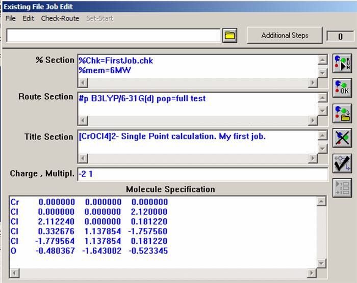
Finally, since the Gaussian input file is always an unformatted text or ASCII file, I would like you to present it in "As-Is" format:
%Chk=FirstJob.chk
%mem=6MW
#p B3LYP/6-31G(d) pop=full test
[CrOCl4]2- Single Point calculation. My first job.
-2 1
Cr 0.000000 0.000000 0.000000
Cl 0.000000 0.000000 2.120000
Cl 2.112240 0.000000 0.181220
Cl 0.332676 1.137854 -1.757560
Cl -1.779564 1.137854 0.181220
O -0.480367 -1.643002 -0.523345
As you can see, there is not much difference in constructing such a file as compared to that written with the help of Gaussian03W interface (but not the GaussView!). Note the blank lines after the command line, title line, and (not visible, but still there!) molecular specification lines.
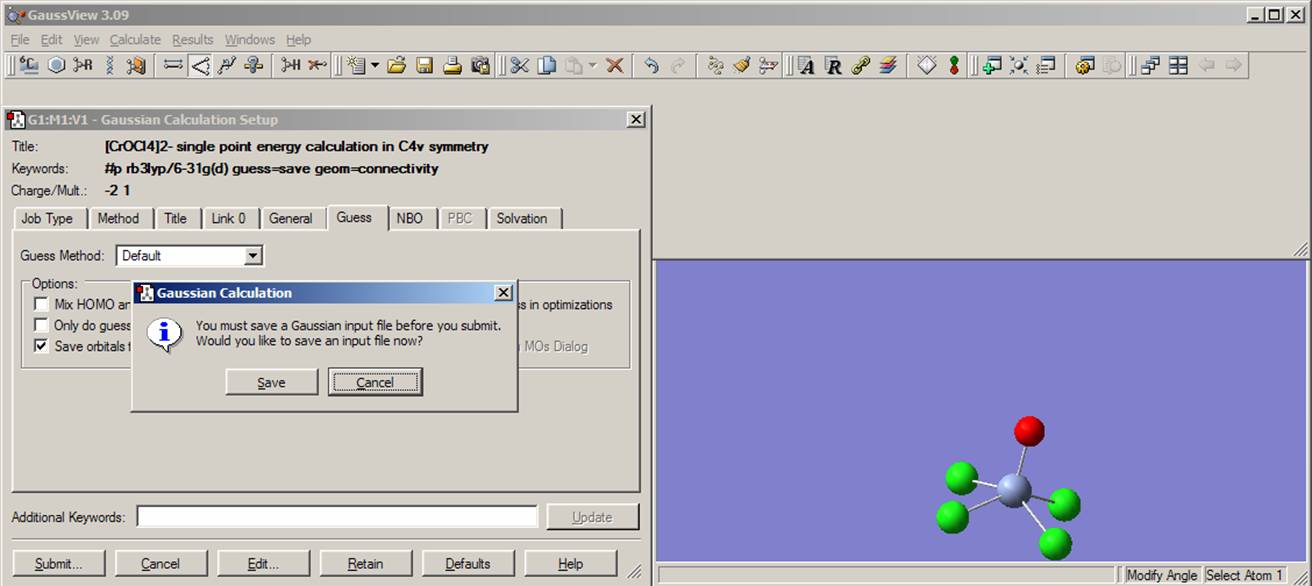
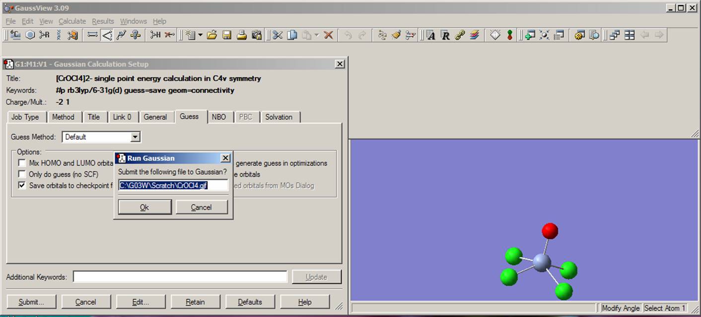 If you are executing a Gaussian03W job from the GaussView interface, click on the submit button. If you didn't save the input file before, the Gaussian03W will ask you to do so. Once the Run Gaussian window appears, click OK.
When you have created your input file - either with Gaussian03W interface or directly using the ASCII text editors, you should save it first. Once you have saved the file, you can run the calculations from the Gaussian03W interface by clicking on the "Run" button located on the top right side of the Gaussian job window:
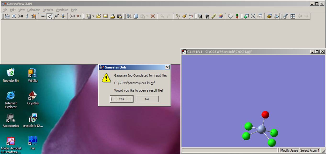
Finally! The computer is doing your job! You can relax for a few seconds.
Gaussian03W writes its plain text output file called the output (generated if you started calculation from Gaussian03W) or logfile (if you started calculation from GaussView or non-Windows OS), which has the same name as the input file, but with the "out" or "log" extension. The full information printed to the output file is very large, but we will focus on information which is useful for this lab. First, open the output file with a text editor (for instance notepad, wordpad, MS Word, FAR, etc.).
First, you will see copyright and citation information on the Gaussian03W program, which is important, but not interesting for our lab. Immediately after these lines, you will see something like the following:
******************************************
Gaussian 03: IA32W-G03RevC.02 12-Jun-2004
22-May-2005
******************************************
This "header" provides you with information on Gaussian03W version and date, when calculations were conducted.
In the next section, your Link 0 and Command Section will be mentioned followed by IOP's lines (we will discuss IOP's on the lecture):
%chk= FirstJob.chk .....................................................................Link 0 section starts from this line
%mem=6MW
%nproc=1
Will use up to 1 processors via shared memory.
--------------------------------------------------
#p rb3lyp/6-31g(d) pop=full geom=connectivity test .......................Command section starts from this line
--------------------------------------------------
1/38=1,57=2/1; ...........................................................................IOP's section starts from this line
2/17=6,18=5,40=1/2;
3/5=1,6=6,7=1,11=2,16=1,25=1,30=1,74=-5/1,2,3;
4/7=1/1;
5/5=2,32=1,38=5/2;
6/7=3,28=1/1;
99/5=1,9=1/99;
Job Title, molecule charge and multiplicity along with the molecular geometry (note that it is presented in the form of Z-matrix in this example) will be echoed in the next section:
----------------------------------------------------------
[CrOCl4]2- single point energy calculation in C4v symmetry.....Job title section starts from this line
----------------------------------------------------------
Symbolic Z-matrix:
Charge = -2 Multiplicity = 1.............................................Charge & multiplicity are mentioned here
Cr................................................................Molecular geometry specification starts from this line
Cl 1 B1
Cl 1 B2 2 A1
Cl 3 B3 1 A2 2 D1 0
Cl 1 B4 2 A3 3 D2 0
O 1 B5 5 A4 2 D3 0
Variables:
B1 2.12
B2 2.12
B3 2.86713
B4 2.12
B5 1.79
A1 85.0963
A2 47.45185
A3 85.0963
A4 107.
D1 -147.40515
D2 -147.40515
D3 106.29743
After this, you will find a lot of details on the current molecular geometry, but I would like to mention only the last block, in which the molecular symmetry and the Cartesian Coordinates (even if you input initial coordinated using a Z-matrix approach) are printed:
Stoichiometry Cl4CrO(2-)
Framework group C4V[C4(CrO),2SGV(Cl2)]
Deg. of freedom 3
Full point group C4V NOp 8
Largest Abelian subgroup C2V NOp 4
Largest concise Abelian subgroup C2V NOp 4
Standard orientation:
---------------------------------------------------------------------
Center Atomic Atomic Coordinates (Angstroms)
Number Number Type X Y Z
---------------------------------------------------------------------
1 24 0 0.000000 0.000000 0.278283..............................Cartesian coordinates are printed starting from this line
2 17 0 0.000000 2.027366 -0.341545
3 17 0 2.027366 0.000000 -0.341545
4 17 0 0.000000 -2.027366 -0.341545
5 17 0 -2.027366 0.000000 -0.341545
6 8 0 0.000000 0.000000 2.068283
---------------------------------------------------------------------
In our example, the stoichiometry is Cl4CrO, charge -2, and the molecular symmetry is C4v. Note that the atomic coordinates, which are located in the three last columns, are in angstroms and atoms are represented by their atomic number (second column).
The next place to have a look is the initial "guess" wavefunction which Gaussian03W generates:
Initial guess orbital symmetries:
Occupied (A1) (B2) (E) (E) (A1) (A1) (E) (E) (A1) (A1)
...........................
(A1) (B2) (E) (E) (B2) (E) (E) (A2) (B1)
Virtual (E) (E) (A1) (A1) (B2) (E) (E) (A1) (A1) (A1)
............................
(B2) (A1)
The electronic state of the initial guess is 1-A1.
First, consider how good your initial "guess" looks. Based on the simple ligand-field theory approach, you would expect that the highest occupied molecular orbital (HOMO) should be a metal-centered dxy orbital of b1 symmetry, while the lowest unoccupied molecular orbital (LUMO) should be doubly degenerate metal-centered dxz,yz orbitals of e symmetry. Your initial "guess" HOMO and LUMO orbitals symmetries (marked in red) are in agreement to the expected one. Second, the electronic state of our system should be 1A1 (you have a diamagnetic molecule!) with agreement to the Gaussian03W generated one.
If everything goes well, a message stating that your wavefunction has converged will appear in the output file:
SCF Done: E(RB+HF-LYP) = -2960.52730107 A.U. after 7 cycles
Convg = 0.6773D-04 -V/T = 2.0025
S**2 = 0.0000
In the first line, you will find the total energy of the system in atomic units. The value to have a look at in the second line is -V/T ratio, which should be close to 2.0. Finally, the S2 value, mentioned in the third line should be zero for diamagnetic systems (we will discuss the S2 value in details in the "Comparison of energies for different spin states in transition-metal complex" lab).
After this section, the orbital symmetries and electronic states of the converged wavefunction will be printed:
Orbital symmetries:
Occupied (A1) (B2) (E) (E) (A1) (A1) (A1) (E) (E) (A1)
....................
(E) (E) (A1) (E) (E) (B2) (E) (E) (A2) (B1)
Virtual (E) (E) (A1) (A1) (B2) (E) (E) (A1) (A1) (A1)
....................
(B2) (A1)
The electronic state is 1-A1.
As you can see, our expected HOMO and LUMO orbital symmetries as well as electronic states look OK.
Since you incorporated the "pop=full" command into the route section line, Gaussian03W will print out all molecular orbital symmetries, energies, and coefficients to the output file:
Molecular Orbital Coefficients
1 2 3 4 5
(A1)--O (B2)--O (E)--O (E)--O (A1)--O
EIGENVALUES -- -215.47484-101.16716-101.16716-101.16716-101.16716
1 1 Cr 1S 0.99639 0.00000 0.00000 0.00000 0.00000
2 2S -0.01195 0.00000 0.00000 0.00000 0.00002
3 2PX 0.00000 0.00000 -0.00001 0.00000 0.00000
4 2PY 0.00000 0.00000 0.00000 -0.00001 0.00000
5 2PZ 0.00000 0.00000 0.00000 0.00000 0.00000
6 3S 0.02617 0.00000 0.00000 0.00000 0.00023
7 3PX 0.00000 0.00000 0.00006 0.00000 0.00000
......................
127 4YZ 0.00000 0.00000 0.00000 0.00002 0.00000
You will use this part of the output file later in this lab. Note that the orbital energies are in atomic units and as you will see later, VMOdes will convert those into eV units.
The next block you will look into is the Mulliken atomic charges:
Mulliken atomic charges:
1
1 Cr 0.432196
2 Cl -0.455739
3 Cl -0.455739
4 Cl -0.455739
5 Cl -0.455739
6 O -0.609239
Sum of Mulliken charges= -2.00000
The sum of Mulliken charges for your molecule is -2 and, as expected, the chromium atom has a positive charge, while both chlorine and oxygen atoms have negative charge. We will discuss different schemes for the charge partition in the lecture.
Next, you will find the calculated dipole moment of [CrOCl4]2- complex:
Dipole moment (field-independent basis, Debye):
X= 0.0000 Y= 0.0000 Z= -1.5469 Tot= 1.5469
In this case, the total dipole moment of the molecule is 1.5469 Debye and it is pointed out from the positive chromium atom toward the more electronegative oxygen. Note that the "X" and "Y" components of dipole moment are zero as should be expected.
Finally, the job cpu time and normal termination line are printed at the end of the output file:
Job cpu time: 0 days 0 hours 0 minutes 32.0 seconds.
File lengths (MBytes): RWF= 16 Int= 0 D2E= 0 Chk= 7 Scr= 1
Normal termination of Gaussian 03 at Sun May 22 21:38:43 2005.
 Now, lets go back to the GaussView program and find out how you can print molecular orbitals. First, open GaussView or accept a file to open command if you run calculation in the GaussView mode. You can open a variety of different files, but the one you are looking for is the binary Gaussian03W checkpoint file, which contains the most detailed information on the molecule you just calculated:
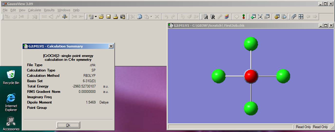 You can see the final energy, structure, and dipole moment by going to the Results menu and clicking on Summary:
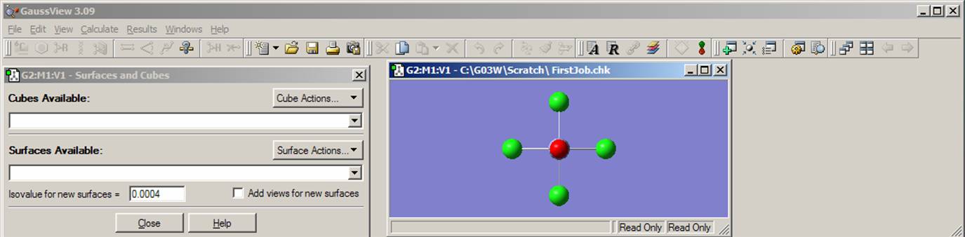
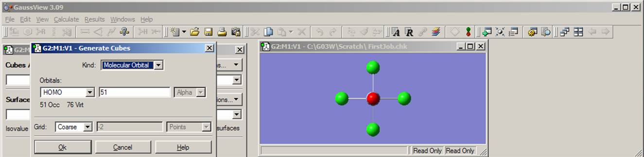 Next, click on Results menu and select Surfaces. Then from the Surfaces and Cubes menu choose Cube Action pop-up menu and go to New Cube. Under Generate Cubes menu choose HOMO (from the Orbitals pop-up menu) and click Ok. There are 102 electrons in your molecule and all orbitals are either doubly occupied or empty. Thus orbital number 51 represents the HOMO. Now relax again and wait until the cube.exe program generates an orbital surface.
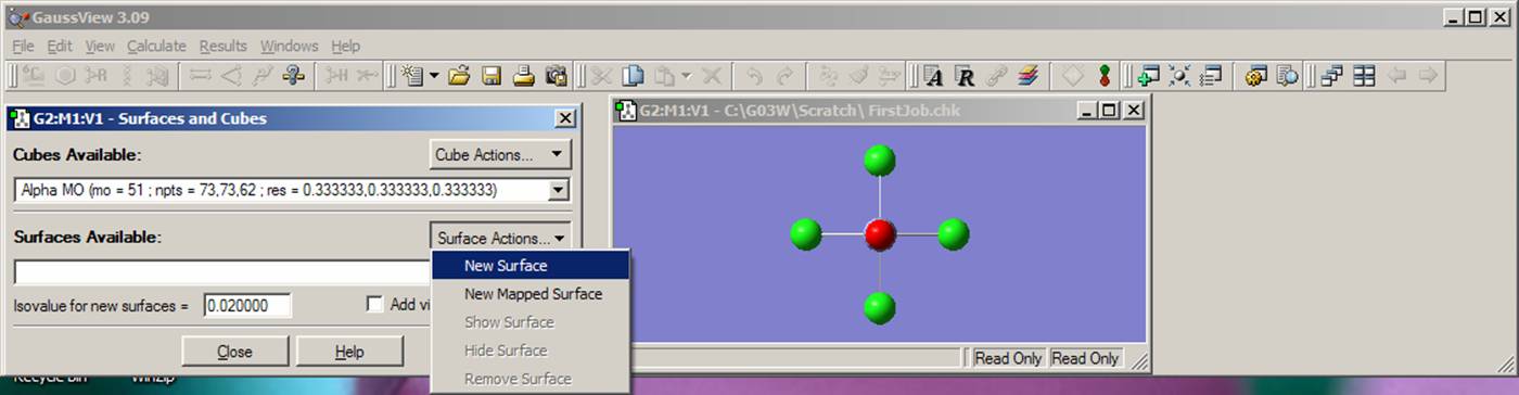
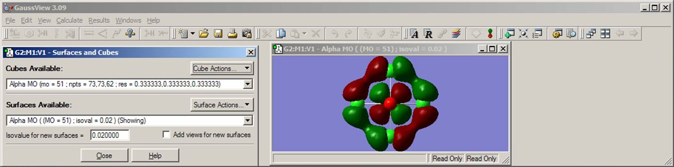 Once the orbital surface is generated, it will appear in the Cubes Available line. Next, you will use the Surface Actions pop-up menu and choose New Surface. An isosurface of the HOMO of the [CrOCl4]2- complex will appear in the molecule containing window. You will see that the isosurface of the HOMO consists of two colors (green and red), which represent the positive and negative isosurfaces. The choice of the color for positive or negative part is arbitrary, so just assign one color to the positive and another to the negative nodes. Now choose the "Save Image" command from the File menu. Save the image of the HOMO. Instead of a solid grid for the isosurface, you can also use mesh grid. Select View menu, click on Display Format, choose the Surface tab and finally select the mesh option. This will change a solid grid to the mesh grid in the plotted HOMO isosurface. Next, go back to Surface Actions pop-up menu and click on the Remove Surface button. This will remove the HOMO from the molecular frame. Following the same procedure, generate and save the LUMO and LUMO+1 orbitals. In the last case, click on Orbital Number from Orbitals pop-up menu and type 53 as the number of orbital. In addition, find predominantly dx2-y2 and dz2 orbitals. Now is the time to analyze HOMO, LUMO, and LUMO+1 orbitals. The HOMO orbital clearly consists of the chromium dxy atomic orbital and four chlorine atom in-plane p-orbitals. Clearly, you can see bonding interactions between chlorine atomic orbitals and anti bonding interactions between chromium and chlorine orbitals. Do the same qualitative observations on the LUMO and LUMO+1 orbitals. By looking at the figure, you can estimate that the chromium dxy atomic orbital contribution into the HOMO is about 20%. How you can prove or disprove this? Simply. You just need to use the VMOdes program to calculate the contribution of the chromium, chlorine, and oxygen atoms into the HOMO, LUMO, and LUMO+1 orbitals. First, go to the VMOdes page and became more familiar with this program. Once you are get the idea of what VMOdes is for, construct data.txt file for your complex:
5
1 Chromium, 1 36
1 Chromium d orbitals, 18 36
1 Cl, 37 112
1 Oxygen, 113 127
1 Total, 1 127
Next (and this is good to know) go to output file and truncate the first five orbital energy values from:
Molecular Orbital Coefficients
1 2 3 4 5
(A1)--O (B2)--O (E)--O (E)--O (A1)--O
EIGENVALUES -- -215.47484-101.16716-101.16716-101.16716-101.16716
1 1 Cr 1S 0.99639 0.00000 0.00000 0.00000 0.00000
2 2S -0.01195 0.00000 0.00000 0.00000 0.00002
To:
Molecular Orbital Coefficients
1 2 3 4 5
(A1)--O (B2)--O (E)--O (E)--O (A1)--O
EIGENVALUES -- -215.4748 -101.1672 -101.1672 -101.1672 -101.1672
1 1 Cr 1S 0.99639 0.00000 0.00000 0.00000 0.00000
2 2S -0.01195 0.00000 0.00000 0.00000 0.00002
Now start VMOdes and generate an output file. Find HOMO, LUMO, and LUMO+1 orbital compositions:
51 (B1)--O 3.722 81.4 81.4 18.6 0.0 100.0
52 (E)--V 6.840 74.4 67.7 12.2 13.4 100.0
53 (E)--V 6.840 74.4 67.7 12.2 13.4 100.0
You can easily see now that our initial thought was completely wrong. Indeed, the HOMO consists of 81.4% of chromium dxy orbital! Do the same analysis for LUMO and LUMO+1 orbitals as well as predominantly chromium-centered dx2-y2 and dz2 orbitals.
Congratulations! You just completed your first Gaussian03W lab. I would encourage you, however, to try a few more different transition-metal containing molecules. Good examples are: paramagnetic [MoOCl4]- (C4v symmetry), and diamagnetic Ferrocene (try both D5d and D5h symmetries, which represent staggered and eclipsed conformations, respectively). You can construct these molecules by yourself or download coordinates of [MoOCl4]- and Ferrocene with D5d and D5h symmetries from this Web-site (please note that you have to request a password to unzip these files).
Good Luck!
University of Manitoba
Department of Chemistry Home Page
© 2004-2017 Victor Nemykin, All Rights Reserved
Last Updated October 02, 2017