TUTORIAL:
Visualizing genomes with DNAPlotter
|
Sept. 12, 2018 |
TUTORIAL:
Visualizing genomes with DNAPlotter
|
Sept. 12, 2018 |
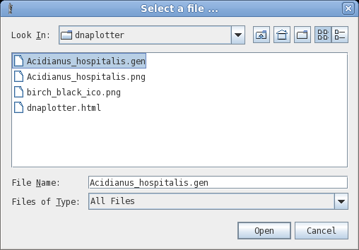
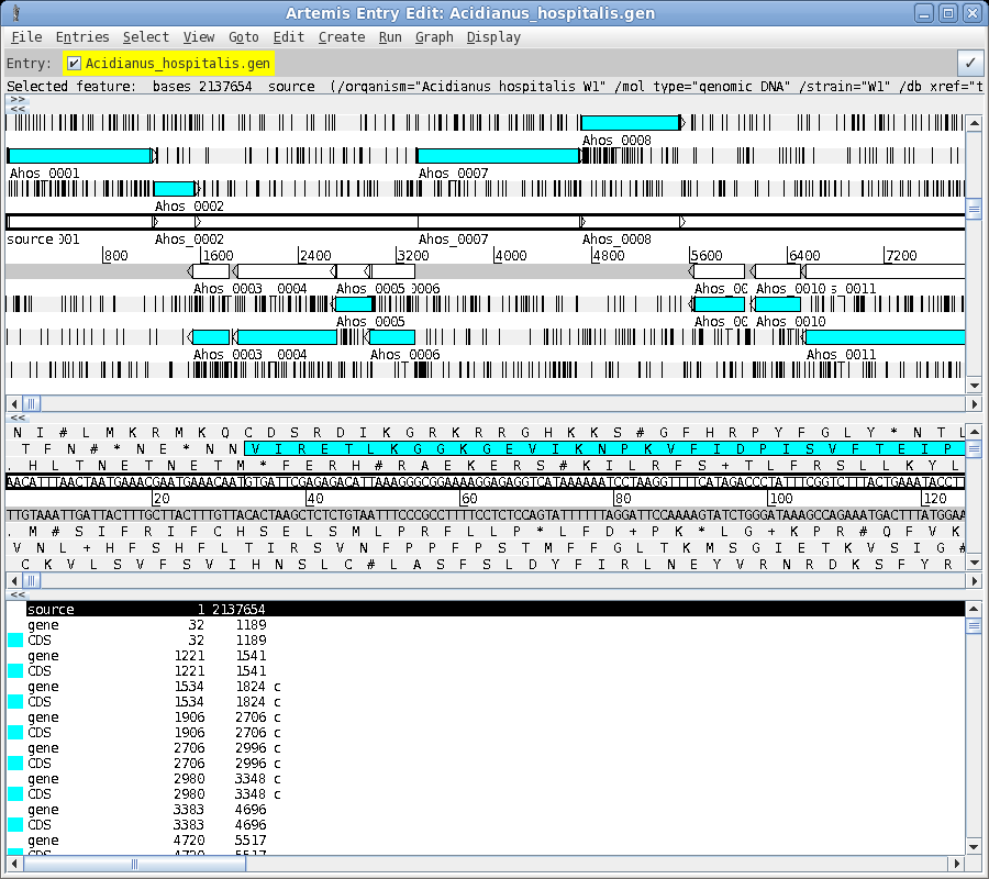
| To read the file, choose File --> Open. Set Files of Type to All Files. Next select Acidianus_hospitalis.gen. This GenBank entry contains the complete genome. Click on Open to open the file. The artemis window should appear something like the one below. |
 |
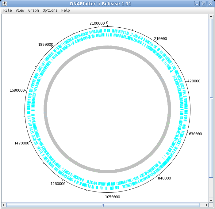
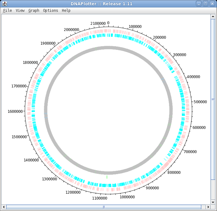
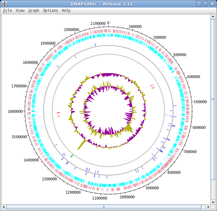
| To launch DNAPlotter, choose File -->
Open in DNAPlotter. The default plot shows, from the outer circle and going inwards:
|
 |
| Changing number and
tick mark intervals When more precision is desired on the scale line, we can change the interval for numbering and tick marks. In DNAPlotter choose Options --> Tick marks. 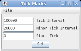 Set Tick interval to 100,000 and the Minor Tick Interval to 20,000 and press Set to apply the changes. |
 |
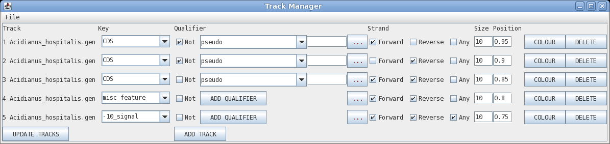
Track: the circle to display, going from outer to inner
Key: display all features with this key
Qualifier: display only features with this qualifier
Not: display only features that do NOT have this qualifier
Elipsis (...) : remove qualifier
Strand: forward, reverse or any
Size: width of the line in pixels
Position: radius at which to display the circle
Colour: brings up a colour menu for the feature
Delete: delete this track
| Let's start by changing the colour of the CDS
sequences displayed on the forward strand (outermost track).
Click on Colour to open the colour chooser. Click on the
color box to the left of the button that says "Apply Colour
to All". |
 |
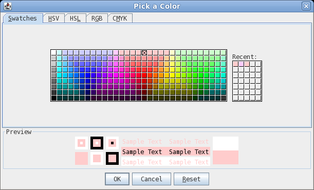
| The colour chooser has five different methods
for specifying a color. For now, we'll use the Swatches
method. In this example, click on one of the pink boxes in the center of the top line. You'll notice that when the mouse hovers over a color, the RGB code for that colour appears (eg. 255,204,204). Click on OK to continue. |
 |
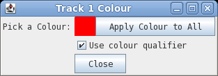
| You MUST click on Apply
Colour to All, at this point, for your colour
change to take effect. If you fail to do so, the default
colour of White will be used, and it will look as if your
circle has disappeared! (This little quirk took me a long
time to figure out.) Next, click on Close to return to the
track manager. |
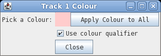 |
| About the "Use colour qualifier" box.
Some genome annotation software an generate annotation files
that include colour codes for each feature. If the use
colour qualifier box is checked, DNAPlotter will use those
colours. An example of such a file is S_typhi.tab,
used in the Hinxton
Artemis tutorial. |
|
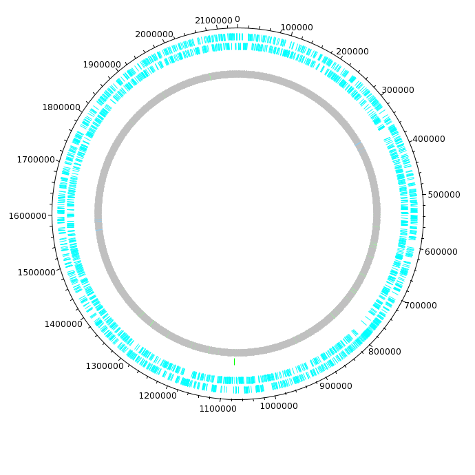
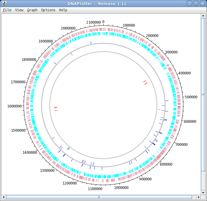
| The DNAPlotter window should now look like
this: Having different colours for the two strands make it easier to distinguish features on each strand. |
 |
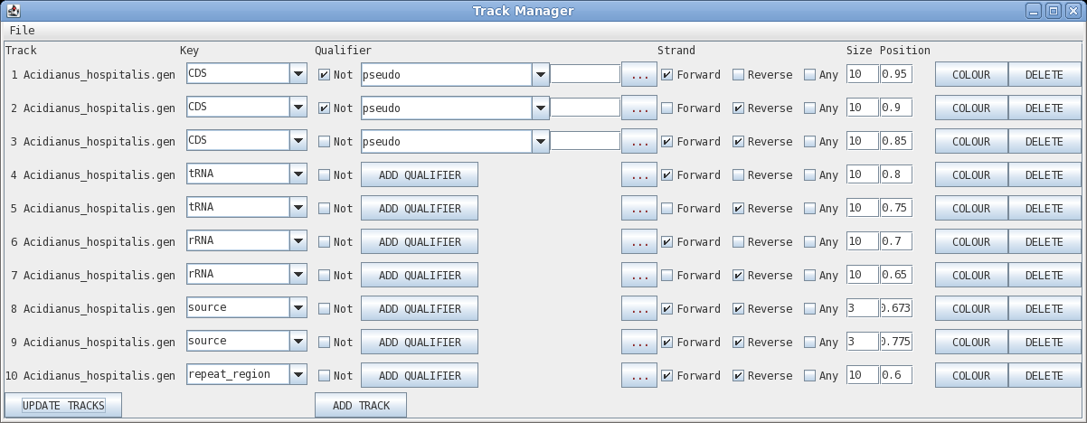
| Click on "Update Tracks" to make your changes
take effect. The map should now appear as shown at right. |
 |
GC plot - tells the fraction of bases that are either G or C within a sliding window, plotted between the minimum and maximum values.
GC skew - tells the degree to which the GC content is skewed toward G or skewed toward C, plotted between teh minimum and maximum values. It is calculated by the formula GC skew = (G - C)/(G + C). (To clarify, G - C is a subtraction. This doesn't refer to GC dinucleotides.) When (G-C) is greater than 0, the bias is toward G. When (G-C) is negative, the bias is toward C.
| The final plot should look similar to that
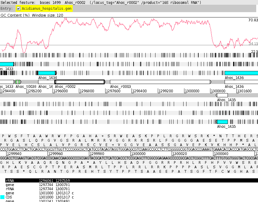
shown at right. At this point, it would be a good idea to save the settings for this map in a file, so that the same settings can be applied to each track in the display of other genomes. In DNAPlotter, choose File --> Export Track Template, and save as Acidianus_hospitalis.tracks. One of the most obvious features that we see in the graph is the spike in GC content in the immediate vicinity of the rRNA genes, shown in green on track 6. At this level of resolution, we can't be sure that the spike perfectly coincides with the rRNA genes. To verify that hypothesis, go back to the Artemis window and go to the neighborhood of the spike at nucleotide 1,300,000: Goto --> Navigator --> Goto Base: 1300000. Next, display the GC plot by choosing Graph --> GC content (%). To more easily distinguish the plot from the average line, move the mouse into the graph, hold down the right mouse button and choose Configure. Click on the Color box to set the color of the plot to red, and click OK. |
 |
To see which genes are under the long peak in GC content, click on the genes marked Ahos_r002 and Ahos_r003. The gene annotation will be highlighted in the feature box at the bottom. We have confirmed that both of these features correspond to gene features at the coordinates of these two ribosomal RNA genes. |
 |
 A word of caution about genome
annotations. A word of caution about genome
annotations.Not everything in a genome is annotated. The features that you see in a genome are limited to those that the authors or annotation pipeline chose to annotate. For example, some projects will annotate repeat regions or transposable elements. Others might annotate nothing except CDS regions. The apparent absence of a feature does not necessarily mean that those features are not present in the genome!! Not everything that is annotated is annotated correctly. Genome annotation is at best an imperfect science. Although most annotations are based in some way on sequence similarity to known genes or features, there are many ways to get both false negatives and false positives. As well, the exact start and stop positions of genome features are not always correctly assigned by automated software. Very few genome features are ever verified by experiments. |