TUTORIAL: PHYLOGENETIC ANALYSIS OF DISCRETE STATE DATA |
Oct. 21, 2014 |
TUTORIAL: PHYLOGENETIC ANALYSIS OF DISCRETE STATE DATA |
Oct. 21, 2014 |
| This tutorial assumes that you have already gone through the DNA phylogeny tutorials at $birch/tutorials/bioLegato/bioLegato.html |
Green foxtail is a grassy weed that is commonly found in cultivated fields in the Canadian prairies. Foxtail is usually controlled in cereal crops by inhibitors of acetyl-CoA carboxylase (ACCase) such as fenoxaprop-P-ethyl or by trifuluralin. However, accessions of foxtail have been identified which are resistant to one or both types of herbicide. The map below indicates the locations of sites in the province of Manitoba where herbicide resistant green foxtail populations have been found.
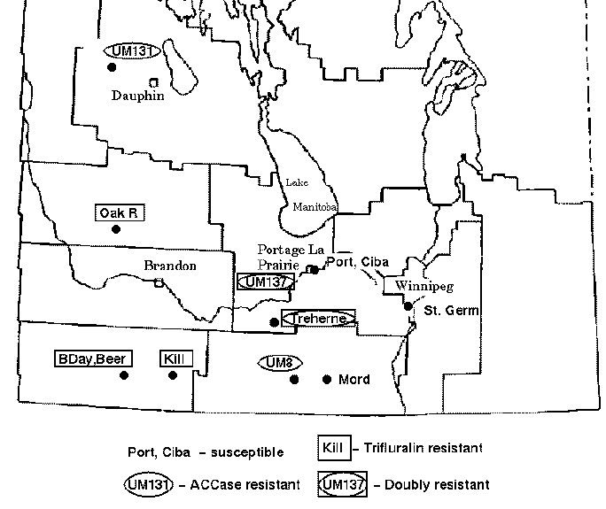
Thirteen accessions of green foxtail were tested for resistance
to ACCase inhibitor and trifluralin. These accessions were also
subjected to RAPD analysis, in which polymorphism was scored at 42
loci. The data are represented in Phylip format in the file manitoba.phyl.
Note: Phylip format for discrete data
|
Create a directory called foxtail, and save manitoba.phyl to this
directory. Start blmarker by typing
blmarker
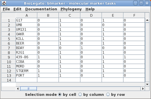
To read this file into blmarker, choose File -> Import Phylip Discrete Data.

The sequences will be read into the blmarker window.
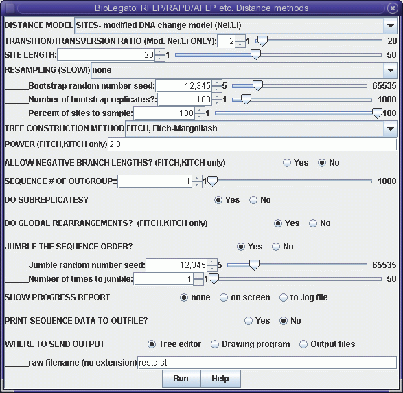
Although this menu is quite the same as the distance menu for DNA and protein sequences, let's look at some important menu items:
DISTANCE MODEL: SITES/REST. FRAGS. - By default, each marker represents a distinct genetic locus. This is true for most types of molecular markers. However, for RFLPs, it is often the case that a given locus may be represented by two distinct bands, representing alleles. If this were restriction fragment data then, "REST. FRAGS." should be used.The output appears in windows as shown:SITE LENGTH - The number of nucleotide positions assayed by a marker method. For RFLP analysis using restriction enzymes with 6-base recognition sequences, this number is 6. That is, cleavage by the enzyme requires specific nucleotides must match at 6 positions. For RAPDs using primers 10 bases long, SITE LENGTH is 20 (not 10!). This is because the primer must match 10 bases on each side of the fragment to be amplified. For AFLPs, the number of selective bases is between 14 - 18 nt, depending on the restriction enzymes used. Obviously, the longer the site length, the lower the probability of a 0 -> 1 mutation. Put another way, it is much easier for a single site to mutate to match a 6 base restriction sequence than it is for two nearby sites to mutate to match a 10 base primer.
OUTFILE (manitoba.fitch.outfile)
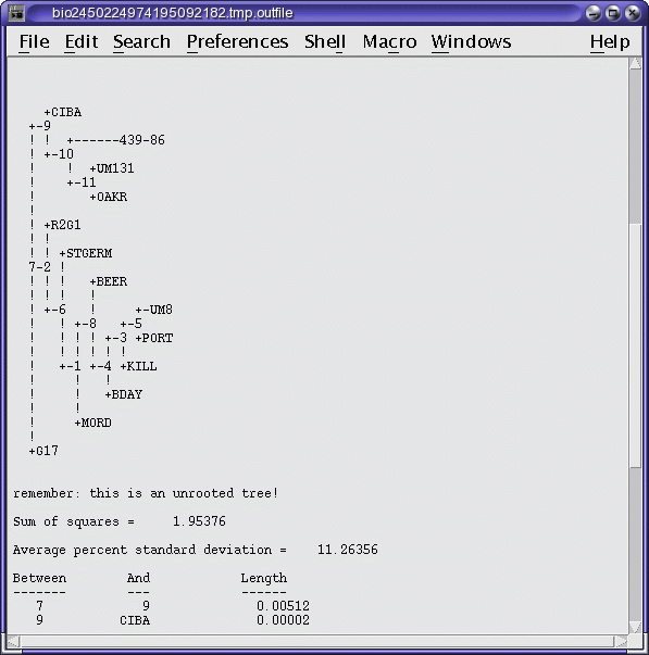
TREEFILE (manitoba.fitch.treefile)
The output treefile is launched in two applications: a text
editor, to make it easy to save the file, and bltree, to make it
easier to work with the tree, or to use various tree drawing
programs.


ATV
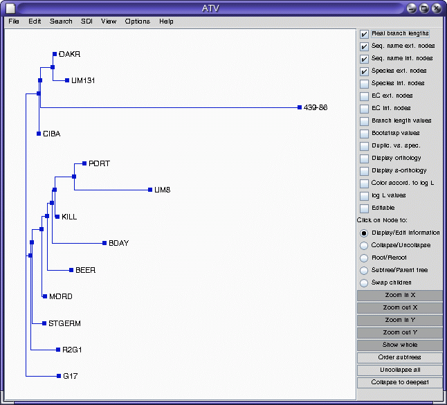
Note that accession 439-86 appears to be an outgroup, very distantly related to all other accessions. This is consistent with the fact that 439-86 originated in China, and was included as a control.
Several parsimony methods are available, as indicated in the
menu:

In this example, Joe Felsenstein's Polymorphism parsimony method has been chosen. This method is worthy of some mention. For most molecular marker systems, Dollop parsimony is usually the most realistic choice because it assumes that the probability of a 1 -> 0 mutation (loss of a band) is much greater than a 0 -> 1 mutation (gain of a band.) However, this model may be overly pessimistic, simply due to the fact that, if polymorphism for a given site exists, in a population (ie. both 1 AND 0 are present), a population containing both alleles might be sampled, and erroneously assigned 0, even though 1 is present in other individuals that were not sampled. Polymorphism parsimony tries to take this possibility into account. If most nodes on a branch contain 0s, but at least one 1 node is implied, the polymorphism parsimony option of dollop will assume that the presence of the 1 is due to polymorphism in the population, rather than a rare forward mutation.
For the same input data, dollop will produce the following output files:
manitoba.polymorphism.outfileMake sure to save your files using these names for the next example.
manitoba.polymorphism.treefile
When a data set is monomorphic at a given site (ie. all 0 or all 1) is it because the population is monomorphic, or is it that we simply haven't sampled enough individuals to detect polymorphism? In a population monomorphic for absence of a band (ie. all 0), probability of seeing a band is zero. In a population containing 1s, if we take a sample that contains all 0's, the probabilty of 1 is most definitely not 0. We only got all 0's due to how the population was sampled. For this reason, restml defaults to No, for All sites detected'. For situations in which some sites may be polymorphic, but are not reflected in the data, however, choose 'Yes', all sites detected. |
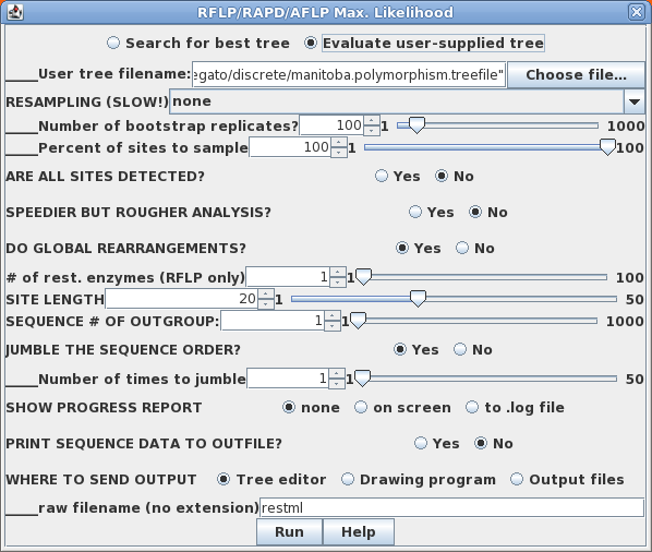 |
Sample output files:
manitoba.restml.outfile
manitoba.restml.treefile
| WARNING
Maximum likelihood methods are very slow, because they attempt to consider an enormous number of possible trees. The time required increases exponentially with the number of sequences. Therefore doubling the number of sequences does not double the execution time. In fact for restml, the time required increases roughly with the 4th power of the number of the sequences! For most practical purposes, direct tree construction with greater than 30 sequences requires prohibitive amounts of time. Since bootstrapping multiplies the time required often by
a factor of 100 or more, we usually don't have the luxury
of bootstrapping with maximum likelihood methods. However,
as illustrated above, we can bootstrap with a less time
consuming method such ase parsimony, and then build the
final tree with Maximum Likelihood. |