Understand how life history can constrain genome size
Define synteny and microsynteny
Understand the purpose of comparative genomics research, and
what it can reveal
Be able to describe and explain the experimental data about
the changes in repetitive sequences
Understand the role of transposons in genome evolution, and
factors that activate them
Know the different possible roles for repetitive elements in
eukaryotic genomes
In introductory genetics, we are presented with linkage maps
that make the eukaryotic genome look like it is cast in concrete.
Indeed, perhaps the most difficult thing for many geneticists to
swallow about transposition was the 'Pandora's box' of genomic
chaos that it implied. Transposition relegated the gene from its
status as a house built upon a rock, to more of a molecular mobile
home. Perhaps it is not entirely a coincidence that not long after
McClintock's publications of transposition, that the model of
plate tectonics shook the science of geology like an earthquake.
The eukaryotic genome has never been the same since. In
retrospect, we can see that evolution requires a fluid, dynamic
genome. Without change, there is no evolution. We can now make
several generalizations regarding genome evolution:
Genome sizes and karyotypes can differ drastically even among
closely-related species. This necessarily demands that fundamental
changes in genome structure can occur over relatively short
evolutionary times.
Most of the changes occur in the middle repetitive
fraction of the genome.
Most of these changes are in non-coding DNA.
Genome size can change relatively quickly in evolution
The sizes of chromosomes in
Crepis species are drawn to scale, accompanied by drawings
of florets and achenes, also to scale.
This
example illustrates how drastically genome size and
chromosome number can change in short evolutionary times.
It
also illustrates something often observed, which is that
the sizes of plant organs such as leaves, stems or fruit
are often larger in species with larger chromosomes.
Fig. 9-19. Species of the
genus Crepis showing the size relations of chromosomes,
florets (lacking ovaries), and achenes, all drawn to the
same magnification so that the sizes are relative to
each other. A. C. sibirica; B, C. kashmirica
; C, C. conyzaefolia; D, C. mungierii;
E, C. leontodontoides ; F, C. capillaris;
G, C. suffreniana; H, C. fuliginosa
(rearranged from Babcock, 1947). from Cytogenetics
- the chromosome in division, inheritance and
evolution. Carl P. Swanson, Timothy Merz and
William J.Young. 2nd Edition. Prentice-Hall. Chapter 9.
Evolution of the karyotype.
achene
(əkēn')
, dry, simple, one-seeded fruit with the seed attached
to the inner wall at only one point. Achenes are
indehiscent, i.e., they do not split open at maturity.
The so-called seed of a sunflower is an achene; the
shell is the wall of the fruit, and the true seed lies
within. A strawberry consists of many achenes embedded
in a fleshy receptacle.
Genome Size is Related to Life History
The time required for mitosis
and meiosis increases with genome size.
Table 9.6. Duration of mitosis and
meiosis in a number of plant species, together with their
DNA values in picograms and their annual or perennial
habit; where the DNA values are different, both are given.
Species
Picograms per Haploid
Genome
Mitosis in Hours
Meiosis in Hours
Plant Habit
Crepis
capillaris
1.20
10.8
--
Annual
Haplopappus
gracillis
1.85
10.5
36.0
Annual
Pisum
sativum
3.9,
4.8
10.8
--
Annual
Ornithogalum
virens
6.43
--
96.0
Perennial
Secale
cereale
8.8,
9.6
12.8
51.2
Annual
Vicia
faba
13.0,
14.8
13.0
72.0
Annual
Allium
cepa
14.8,
16.25
17.4
72.0
Perennial
Tradescantia
paludosa
18.0
18.0
126.0
Perennial
Endymion
nonscriptus
21.8
--
48.0
Perennial
Tulipa
kaufmanniana
31.2
23.0
--
Perennial
Lillium
longiflorum
35.3
24.0
192.0
Perennial
Trillium
erectum
40.0
29.0
274.0
Perennial
Source: Van't Hof, 1965, and Bennett, 1972.
You might think that genome size shouldn't affect mitotic cycle
time. If the number of replication origins per Mb stays the same,
all genomes should replicate at the same rate. Therefore, there
must be other limiting factors eg. nuclear or cytoplasmic volume
probably doesn't double when genome size doubles. Therefore, the
concentration of dNTPs could be a major limiting factor.
Annuals tend to have
smaller genomes and shorter mitotic cycles. Perennial plants
tend to have larger genomes and longer cell cycles.
Annuals have to grow
very rapidly in spring. Therefore, ecological competition forces
annuals to have smaller genomes.
Question: Is the
perennial habit more tolerant of a longer mitotic cycle? What is
the advantage of a larger genome or longer mitotic cycle?
Bigger organs means
more biomass utilized, which means more biomass needed. Big
genomes are probably better tolerated when habitat is not
limiting eg. food, water, light, space. The prediction would be
that small genomes are favored under limiting conditions. This
may be why our crops have big genomes. We pamper them with a
good environment. Domesticated crops are poor competitors
outside of cultivation.
Take home
lesson: Genome evolution can be constrained by life history.
Allopolyploids are the result of speciation by interspecific
hybridization
evolution - The change in
allele frequencies within a population. This definition could
encompass any genetic change, from single point mutations, to
major chromosomal rearrangements.
speciation - The evolutionary process by which two
populations diverge, resulting in decreased ability to
hybridize. As populations diverge genetically, reproductive
barriers arise, preventing mating, interfering with meiosis, or
resulting in hybrids that are less fit than progeny from
within-population matings. When fertile progeny can no longer
result from matings between two populations, speciation can be
said to be complete.
Speciation is not necessarily a sudden
event. Although every speciation event is probably a special
case, in general speciation is brought about through reproductive
isolation and genetic divergence. Reproductive isolation can be
the result of geographical or physical separation of populations,
or due to divergence of chromosome structure or number. In turn,
genomic changes can serve as barriers to interbreeding between two
populations. Eventually, enough divergence has occurred that
interbreeding is impossible. It is at this point that, strictly
speaking, two distinct species exist.
However, taxonomists often
define phenotypically distinct populations as species, even when
reproductive barriers are not complete. On the one hand,
the greater the genetic divergence between two species, the
lower the fertility rate will be in interspecific hybrids.
On the other hand,
when interspecific hybridization does occur, it can often
result in the creation of a new species, distinct from the
parental species.
The creation of allopolyploid
species is through interspecific hybridization between
morphologically distinct diploid species, with retention of both
chromosome complements. This effectively doubles the genome size
C and the chromosome number n.
(amphidiploidy= allopolyploidization)
Determination of ancestral species
can be made based on geographical distribution, morphological
features, chromosome counts, karyotype analysis, isozyme banding
patterns and molecular studies.
Putative ancestors can be verified
through interspecific hybridization, synthesis of
allopolyploids, comparison of morphological traits, meiotic
pairing and fertility in the allopolyploids and their hybrids.
Example: the genus Brassica
The genus Brassica consists of three elementary or basic genomes
Brassica campestris, or Brassica rapa (A;
n=10), B. oleracea (C; n=9), and B. nigra (B;
n=8). These diploids are secondary polyploids from an extinct
species with a basic chromosome number of x=6, based on pachytene
chromosome analysis in the haploid genomes. If 1-6 represent the
ancestral basic six chromosomes, the following represents
individual diploid genomes' complement of these basic six
chromosomes.
Comparison of chromosomal complements of Brassica
spp.
Species
Genome
N
Haploid complement
Polysomy?
B. rapa
A
n=10
11 2 3 44 5 666
Double tetrasomic and hexasomic
B. nigra
B
n=8
1 2 3 44 5 66
Double tetrasomic
B. oleracea
C
n=9
1 22 33 4 55 6
Triple tetrasomic
B. rapa x B. nigra
AB
n=18
111 22 33 4444 55 66666
U (1935) demonstrated the genome
relationships by studying the meiotic chromosome pairing in
triploid hybrids
Resynthesis of B.carinata - 2n= 34 BB CC by
hybridizing B. nigra BB and B. oleracea CC
followed by doubling produced an amphidiploid BB CC with 0 to 4 IV
(tetravalents) and 9 to 17 II (divalents) at metaphase I
followed by a nearly normal second meiosis and some production of
fertile pollen. Another synthesis ofB.carinata showed a normal meiosis
with 17 II
and high seed fertility.
Resynthesis of B.napus and
B.juncea -
normal meiosis, resemble the 'natural' allo-tetraploid species and
are fertile. The 'natural' allotetraploids have a more stable
meiotic behavior than the newly synthesized amphidiploids,
presumably due to selection pressure.
Evolution of chromosomes
Based on what we have already discussed in previous lectures, we
can summarize the chromosomal changes that contribute to genome
evolution:
amplification
and deletion of repetitive sequences
deletions
duplications
inversions
translocation
transposition
polyploidy
All of these may contribute to mispairing of hybrids in meiosis,
which represents a reproductive barrier. Reproductive barriers
therfore drive speciation. Once two populations are reproductively
isolated, each population will accumulate further mutations, until
hybridization is no longer possible.
Chromosomal rearrangements seem to characterize differences
between closely related species
Fig.
3-D from Schröck, E. et al. (1996) Multicolor spectral
karyotyping of human chromosomes. Science
273: 494-497.
Even between primates such as
gibbon and man, a large number of chromosomal rearrangements are
evident. In the figure, chromosome painting of gibbon
chromosomes with a human chromosome painting kit shows that all
gibbon chromosomes hybridize with human sequences. However, most
chromosomes exhibit many colors, indicating that sequences
homologous to several human chromosomes are present in each
gibbon chromosome. This experiment illustrates the point that
genomes can differ substantially, even between very
closely-related species.
The longer two species are
reproductively isolated, the more chromosomal rearrangements
each species will accumulate. Thus, chromosomal rearrangements
are an important component of genome divergence, as species
diverge.
As speciation progresses and species diverge, chromosomal
rearrangements, deletions and duplications cause genomes to
diverge. Given enough time, one would expect that the order and
location of genes would become completely different, between
distantly related species. However, even between distantly-related
species, short regions of conserved chromosomal segments, or microsynteny,
can be recognized. A comparison of several grass genomes showed
substantial microsynteny near the adh1 locus in sorghum, maize and
rice. While gene order was conserved, the intervening DNA showed
numerous insertions/deletions of both genes and non-coding DNA.
These results show that it is possible for gene synteny to be
maintained even though the distances between genes can get larger
or smaller.
Take home lesson: As two
species become more and more diverged, meiotic pairing
becomes more and more complex. This results in decreased
fertility of hybrids.
1.
Microsynteny - conservation of genes over short chromosomal
regions
As speciation
progresses and species diverge, chromosomal rearrangements,
deletions and duplications cause genomes to diverge. Given
enough time, one would expect that the order and location of
genes would become completely different, between distantly
related species. However, even between distantly-related
species, short regions of conserved chromosomal segments can be
recognized.
Bennetzen JL, Ramakrishna W (2002) Numerous
small rearrangements of gene content, order and orientation
diffferentiate grass genomes. Plant Mol. Biol.
48:821-827.
A comparison of several grass genomes showed
substantial microsynteny near the adh1 locus in
sorghum, maize and rice. While gene order was conserved, the
intervening DNA showed numerous insertions/deletions of both
genes and non-coding DNA. These results show that it is
possible for gene synteny to be maintained even though the
distances between genes can get larger or smaller.
# - gene lost from
maize adh1, relative to sorghum
* - genes acquired by sorghum adh1 region
Boxes with arrows indicate known or predicted genes
Take
home
lesson: Drastic gain or loss of interspersed repetitive
sequences can take place between genes, without disturbing
the order of genes on a chromosome.
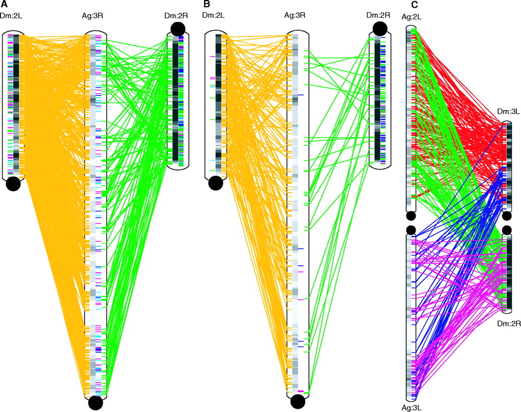
2.
Comparison of the Drosophila and mosquito genomes
shows large blocks of synteny, and partial polyploidization
events.
A - 1:1 orthologs.
Gold and green lines indicate matchups between orthologous
genes in Dm chromosome arms 2L and 2R with Ag chromosome 3R.
This is a gene-by-gene comparison between chromosomes (ie.
each line represents a gene for gene match).
B - microsynteny
blocks. Blocks of known loci conserved between Drosophila
and Anopleles are indicated in gold and green lines.
Blocks indicate groups of genes that are in the same
order when compared between two chromosomes (ie. each line is
a match between microsyntenic blocks).
Both arms of Drosophila
chromosome 2, designated 2L and 2R, have a largely conserved
gene order, when compared to chromosome 3R of Anopheles.
The fact that many of the lines
cross indicates probably at least two ancient inversion
events. This is easier to see in B.
The fact that both 2L and 2R are
roughly colinear with 3R suggests that Drosophila
chromosome 2 resulted from a Robertsonian translocation* of
one copy of chromosome 2 to another.
Although gene order is largely preserved between Ag3R and
the two arms of Dm2, the distance between genes appears to
be greater. This suggests that either Ag3R gained a lot of
repetitive DNA, interspersed between genes, or Dm2 lost a
lot of interspersed repetitive DNA.
C - More complex
relationships between Ag arms 2L and 3L with Dm arms 3L and
2R. Each block of orthologous loci is indicated by red, green,
purple or magenta lines.
Gray bars indicate gene density in a
sliding window of 1 Mb.
Anopheles chromosomes have larger
gene-poor regions than Drosophila chromosomes
Microsynteny between Ag2L and Ag3L, with Dm3L and Dm2R
indicate even further duplications of chromosome arms.
Eukaryotic
genomes often contain lots of hidden polyploidy!
C.
Allopolyoploidization can cause reproducible changes in genome
size, not accounted for by the adding the sizes of the two
genomes together
H. Ozkan,
M. Tuna, and K. Arumuganathan (2003) Nonadditive Changes in
Genome Size During Allopolyploidization in the Wheat
(Aegilops-Triticum) Group. Journal of Heredity 94:260-264
The accompanying table shows data from an experiment in which
various relatives of wheat were crossed, followed by selfing, to
create amphiploid hybrids. The amount of DNA in nuclei was
measured by flow cytometry of chromosomes. DNA amounts are given
in picograms (pg) per nucleus.
Parents and amphiploids
Generation
2n
Genome
Observed DNA value
(pg)
Expected DNA value
(pg)
T.
turgidum ssp. carthlicum
28
BBAA
23.64 ± 0.23
Ae.
tauschii
14
DD
10.16 ± 0.02
T.
turgidum ssp. carthlicum–Ae. tauschii
S1
42
BBAADD
32.13 ± 0.13
33.80
S2
42
BBAADD
31.23 ± 0.06
33.80
S3
42
BBAADD
31.44 ± 0.06
33.8
T.
turgidum ssp. dicoccoides
28
BBAA
23.97 ± 0.04
Ae.
tauschii
14
DD
10.16 ± 0.06
T.
turgidum ssp. dicoccoides–Ae. tauschii
S2
42
BBAADD
31.80 ± 0.11
34.13
Ae.
longissima
14
SlSl
14.35 ± 0.09
Ae.
umbellulat
14
UU
10.87 ± 0.11
Ae.
longissima–Ae. umbellulata
S2
28
SlSlUU
23.21 ± 0.04
25.22
Ae.
sharonensis
14
ShSh
14.65 ± 0.07
Ae.
umbellulata
14
UU
10.80 ± 0.09
Ae.
sharonensis–Ae. umbellulata
S1
28
ShShUU
23.15 ± 0.06
25.45
S3
28
ShShUU
23.17 ± 0.10
25.45
T.
turgidum ssp. durum
28
BBAA
23.91 ± 0.12
Ae.
sharonensis
14
ShSh
14.66 ± 0.07
T.
turgidum ssp. durum–Ae. sharonensis
S3
42
BBAASS
36.52 ± 0.10
38.57
T.
urartu
14
AA
11.76 ± 0.07
Ae.
tauschii
14
DD
10.16 ± 0.13
T.
urartu–Ae. tauschii
S1
28
AADD
19.67 ± 0.26
21.92
S2
28
AADD
19.80 ± 0.07
21.92
S - selfing
generations
Key observations:
a) The observed DNA value in hybrids is always about
2 pg less in hybrids than would be expected by simply adding the
genome sizes of the parents.
b) The loss of 2 pg seems to be consistent and
reproducible, in many crosses. This implies some sort of
programmed response
Possible mechanisms:
non-homeologous pairing resulting in chromosome
breakage, followed by loss of part of one or more chromosomes.
Nulli/tetrasomy
mobilization
of transposable elements
Evolution of interspersed repetitive DNA
Flavell, R.B., Rimpau, J. and Smith, D.B.
(1977) Repeated sequence DNA relationships in four cereal
genomes. Chromosoma
63:205-222.
We can think of the process of speciation as beginning with the
reproductive or geographical separation of two populations of a
species. Initially, the two populations have essentially
identical genomes. Over time, mutational events, ranging
from point mutations to chromosomal aberations to
polyploidization occur. As two species diverge from a common
ancestor, the percentage of sequences shared by both species
decreases, as each species independently gains some sequences
and loses others.
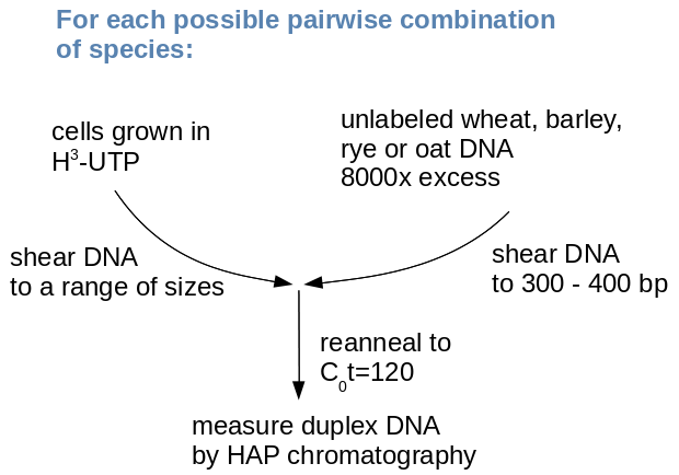
C0t analysis
is a powerful method for measuring the percentage of sequences
shared between two genomes. If DNA from a single species is
allowed to reanneal, essentially all of the DNA should reanneal
if hybridization is allowed to go to completion. If DNA from two
closely-related species is hybridized, one would expect less
than 100% reannealing. The more distantly -related two species
are, the lower the percentage of the DNA that should reanneal.
Specific subsets of repetitive DNA can be amplified or deleted
The relationships
betwee four cereal species, in order of divergence from
a single common ancestor, are shown at right. For
example one speciation event separated the ancestor of
oats, from the common ancestor of barley, wheat and rye.
A later speciation event separated the ancestor of
modern barley from the common ancestor of wheat and rye.
A third speciation event separated wheat and rye into
distinct species.
Once they diverge as separate species, genomic sequences
accumulate mutations. As well, some repetitive sequences
are lost, while new repetitive sequences may arise.
Thus, the set of repetitive sequences in these genomes
would be expected to become more and more different,
with time since speciation.
We can define several
categories of genomic sequences in cereal species:
Group I sequences - present
in all cereals
Group II - barley, wheat & rye, but not oats
Group III - wheat & rye
Group IV - wheat only
Group V - rye only
Group VI - barley only
Group VII - oats only
The more sequences two DNA samples share in common, the higher
the percentage of DNA that should hybridize, between two species.
We can take advantage of this to calculate the percentage of each
of the Group I through VII sequences in each of the four species.
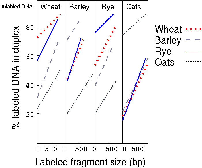
Experimental
design
An excess of unlabled DNA from each of the
four species was hybridized with a range of labeled probes.
The probes consisted of in-vivo labeled DNA, extracted from
cells in culture which were fed radio-labeled nucleotides.
Labeled DNA was sheared to a range of size classes, up to
1000 bp. In separate C0t experiments, each probe
was hybridized with unlabeled DNA from one of the four
species
An interesting observation from this experiment was that percent
duplexed DNA (an indication of relatedness) increased with an
increase in fragment size. Researchers interpreted this to mean
that repetitive DNA was interspersed with single-copy DNA.
"Since duplexes formed from randomly-sheared
fragments frequently have single stranded tails, better
estimates of the proportions of the labelled DNAs in the
renatured conformation come from extrapolations of the
curves in Figure 2 to the ordinate"
[Davidson, et al., (1973)
J. Mol. Biol. 77:1-23.]
If single-stranded tails are present, you would be
overestimating the amount of duplexed DNA. Thus, extrapolating to
0 length fragments solves this problem.
Based on the known ancestries of the four species, we can say in
advance which classes of repetitive families are found in each:
Cereal species and families of repetitive sequences
Cereal
Group I
Group II
Group III
Group IV
Group V
Group VI
Group VII
Wheat
✔
✔
✔
✔
Rye
✔
✔
✔
✔
Barley
✔
✔
✔
Oats
✔
✔
To calculate the percentage of each class in a given species, we
subtract the inter-species hybridization result, as measured at
the Y-intercept, from the within-species result.
"For example, the intercept value when labelled wheat
was hybridized to unlabelled oats DNA is 22%. Group I in wheat is
therefore 22%. The intercept value in the labelled
wheat+unlabelled barley DNA curve is 32%. Group II in wheat is
therefore 32-22=10%. The intercept in the labelled wheat+rye DNA
curve is 58%. Group III in wheat is therefore 58-32=26%. The
intercept in the labelled wheat+unlabelled wheat DNA curve is 74%.
Group IV in wheat is therefore 74-58=16%."
Percentage of each class of repetitive DNA in different
cereal species
Cereal
Group I
Group II
Group III
Group IV
Group V
Group VI
Group VII
Wheat
22 (3.8)
10 (1.7)
26 (4.5)
16 (2.8)
-
-
-
Rye
19 (1.6)
19 (1.6)
14 (1.15)
-
22 (1.8)
-
-
Barley
20 (1.1)
23 (1.3)
-
-
-
28 (1.8)
-
Oats
17 (2.2)
-
-
-
-
-
58 (7.7)
Some specific families of middle repetitive sequences show high
variation
Between species of the same genus, certain middle repetitive
families can vary greatly. In Drosophila, most
individual species possess a different combination of the middle
repetitive families, with the effect that very few families are
present in all the species. In an experiment, D. melanogaster
cloned repetitive sequences were used as a probe against DNA from
other Drosophila species.
Figure 1. Restriction fragments of genomic
DNA from adult D. melanogaster (D. mel), D. erecta (D. ere),
D. yakuba (D. yak), D. simulans (D. sim), and D. mauritiana
(D. mau) hybridized to 32P-labeled repetitive cloned
segments of D. melanogaster, pDm 366, pDm 274, and pDm 73.
Total genomic DNA was digested with Eco R1, fractionated by
electrophoresis on an 0.8% agarose gel, and transferred to
nitrocellulose. Numbers on the left give the length in kb of
HindIII fragments of phage lambda.
From: Dowsett, A. P. (1983) Closely related
species of Drosophila can contain different libraries of
middle repetitive DNA sequences. Chromosoma 88:104-108.
Each probe detects a different middle repetitive sequence. pDm366
detects a sequence that is present in several copies in D.
melanogaster, but not present in other speices. pDm274 detects a
sequence that is present in high copy number in D. melanogaster and
D. erecta, but not in other species. pDm73 detects a sequence that
is middle repetitive in D. melanogaster and D. simulans , but
single-copy in other species.
In fact, some of these middle repetitive elements are transposons:
Figure 2 A,B. Restriction fragments of adult
DNA from five species digested with HinfI and hybridized to
clones containing copia (A) and 412 (B). In situ
hybridization showed that these stocks possess the following
number of copies of copia: D. melanogaster , 10±2; D.
simulans, 4±1; D. mauritiana, 4±1; D. yakuba, 0; and D.
erecta, 0; and the following number of copies of 412: D.
melanogaster, 24±4; D. simulans , 12±2; D. mauritiana, 9±2;
D. yakuba, 3±1; and D. etecta, 0. The two lanes of D. yakuba
DNA are from different stocks. Numbers on the left give the
length in kb of HaeIII fragments of Phi-X 174
Take
home lesson: A repetitive sequence that is present in one
species may not be detectable, or be present in low copy number,
in related species. "Individual mid. rep. families are highly
unstable components of the Drosophila genome
over short periods of evolutionary time."
Transposons play a larger role in evolution than originally
thought
Let's return to transposons, which we
introduced a little while ago in the section on changes in
chromosome structure. Transposons are mobile elements that can
essentially copy and insert themselves into different places in a
chromosome, along with the help of some activator gene. First
discovered in maize by Barbara McClintock, they usually make up a
large percentage of plant and animal genomes.
Transposons are a major component of plant genomes
Raja Ragupathy, Frank M. You, Sylvie Cloutier,
Arguments for standardizing transposable element annotation in
plant genomes, In Trends in Plant Science, Volume 18, Issue 7,
2013, Pages 367-376, ISSN 1360-1385,
https://doi.org/10.1016/j.tplants.2013.03.005.
(http://www.sciencedirect.com/science/article/pii/S1360138513000587)
The data in Table 1
bring out a number of important points:
Transposable
elements make make up a large percentage of most plant
genomes, although there is a great deal of variation between
species.
Class I elements go
through an RNA intermediate. They are transcribed into
RNA, reverse-transcribed into dsDNA, and then inserted into
random sites in the chromosomes.
Class II elements
transpose as dsDNA.
In most plant
species, Class I elements are more prevalent than Class II
elements
The examples of
Cotton and Foxtail Millet demonstrate that even between
different lines of the same species, there can be substantial
differences in the transposon content of the genome. This
suggests that major gain or loss of transposable elements can
occur in a very short time.
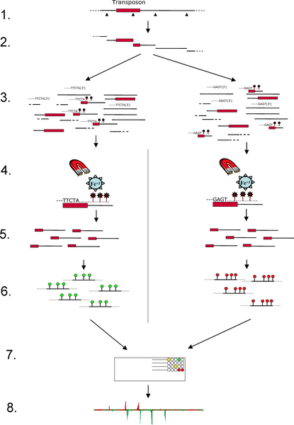
Transposons mobilize in short evolutionary time frames
As a proof of concept experiment, the authors developed an
approach to use microarrays to detect the locations of transposons
in yeast. This method was tested on two yeast strains whose
genomes have been fully sequenced, and the locations of
transposons identified from the sequence. Microarrays were
designed with oligonucleotide probes from unique sequences, spaced
roughly every 300 bp throughout the genome. The results verify
that the the locations of almost all annotated transposons were
correctly identified.
Step One: Isolate regions flanking transposable element
insertions
1. Digest yeast genomic DNA with a restriction enzyme known
to cut within transposons Ty1 and Ty2.
2. DNA samples from 2 strains RM11 and S288c.
3. Many fragments have a partial transposon at one end and
regions flanking the insertion at the other end.
4. Denature DNA and use transposon-specific primer to
synthesize DNA containing biotinylated nucleotides.
Biotinylated fragments are purified by mixing with
streptavidin-coated magnetic beads. Biotinylated DNA is bound
by streptavidin, and magnetic beads are washed to remove
unbound DNA. After washing, biotinylated DNA is released from
the beads by washing in a buffer. The resulting purified
sequences are enriched for unique sequences which flank
transposon insertions.
5. Sequences are labeled with fluorescently labeled
nucleotides: RM11 - Cy3 (green); S288c - Cy5 (red)
6. Mix labeled DNAs and hybridize with a yeast microarray
containing unique yeast probes. Probes have been designed so
that they do not contain Ty1 and Ty2 sequences any other
repetitive sequences Consequently, probes will only hybridize
based on the unique flanking regions from the labeled DNA.
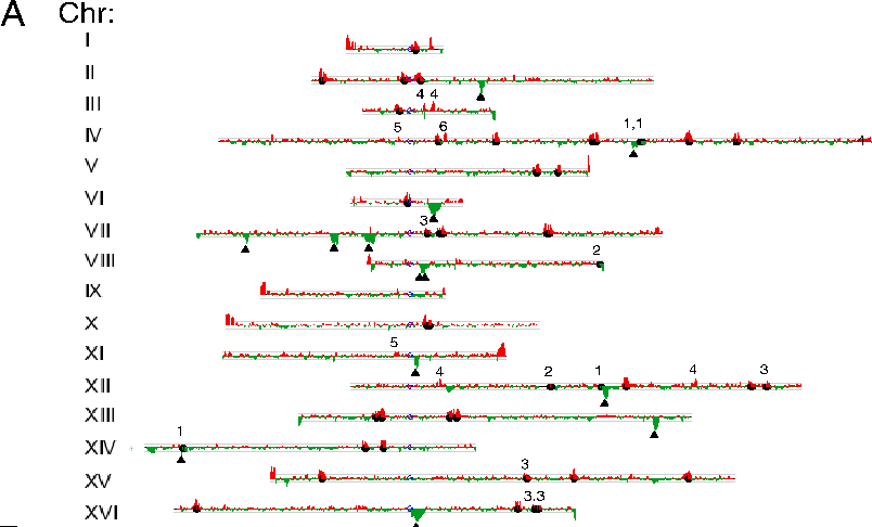
7. Results are superimposed on chromosome maps.
Red Peaks: Ty1
or Ty2 unique to S288c Green Peaks: Ty1
or Ty2 unique to RM11 Black circles: full
length Ty1 or Ty2 elements identified from S288c genomic
sequence Triangles: full length
Ty2 elements identified from RM11 genomic sequence 1,2,3,4
- false negatives 5,6 -
false positives
Red
Peaks: Ty1 or Ty2 unique to S288c Green Peaks: Ty1 or Ty2
unique to RM11 Black circles: full length Ty1 or Ty2
elements identified from S288c genomic sequence Triangles:
full length Ty2 elements identified from RM11 genomic
sequence 1,2,3,4 - false negatives 5,6 - false positives
Step Two: Identify differences in transposon location between
yeast strains
These data
show that even between strains, tremendous rapid changes in the
locations of transposons can occur. The differences in the locations of transposons between
the two strains provide evidence that locations and numbers of
transposons in yeast can change, genome wide, over very short
evolutionary time scales.
Transposons are activated by stress
In most species, transposition is suppressed by epigenetic
imprinting. Methylation of carbon residues prevents mobilization
of transposons, which results in genome stability across
generations. Methylation patterns are known to be inherited from
one generation to the next in most higher eukaryotic species.
Barbara McClintock first observed that what we now know to be the
suppression of transposition is relaxed during stress, resulting
an a de-repression of transposition.
Table 2 shows that there are many
stress conditions which can mobilize transposons,
including:
heat stress
UV light
desiccation
allopolyploidization
passage through tissue culture
osmotic stress (salt stress)
irradiation
wounding
microbial infection
As well, mutations in methyltransferases and even the genetic
background of plants in a cross can induce mobilize transposons.
Why have so much repetitive DNA?
The amount of repetitive DNA present in eukaryotic genomes seems
almost excessive. What's the point of having so much repetitive
DNA? Especially the repetitive DNA that is non-coding! Although
repetitive DNA (particularly highly-repetitive fractions) does not
contribute by coding for a protein, it has other functions for the
eukaryotic cell.
Middle repetitive DNA makes it easier to generate genetic
diversity while decreasing the potential risks of recombination
Genetic diversity can be generated by unequal
crossing over. If there are two copies of a gene, some
crossover events can lead to duplication of the gene on one
chromosome, and deletion on the other. Successive
duplication or deletion of copies can lead to increases or
decreases in the size of multigene families.
If a gene duplication does occur, one copy of
the gene is free to mutate, while the other can retain its
original function. This allows evolution to proceed without
the risk of a deleterious mutation, while still being able
to take advantage of beneficial mutations, should they
occur.
Unequal crossing over could have deleterious
effects if it occurs within a coding region. If all
recombination occurred in coding regions, then you would
have a high frequency of inactivation of genes. This may be
tolerated in unicellular organisms (bacteria and fungi) that
have very little repetitive DNA. In this case their high
reproductive rates my be such that, a) even if a fraction of
individuals gets deleterious mutations due to recombination,
the rapid growth rate is sufficient to prevent a population
bottleneck: b) Furthermore, there is probably a selective
advantage for having a small genome if you have a rapid
growth rate.
The roles of some middle repetitive DNA are still unclear
Other proposed functions for middle repetitive DNA are a little
more speculative. By definition, things like matrix attachment
sites, and perhaps sites (if they exist) that govern higher levels
of chromatin packaging, must be present in hundreds or thousands
of copies. Therefore, such sites fall into the middle repetitive
fraction of the genome.
On the other hand, middle repetitive DNA could simply be selfish
DNA. Some sequences may just be more efficiently duplicated by the
cellular machinery that duplicates sequences. Those sequences that
lend themselves to being duplicated by the DNA replication
machinery will tend to propagate throughout the genome. Darwinian
selection operates even at the molecular level. Transposons are a
good example of selfish DNA.
Middle repetitive DNA might play no significant role at all. Not
everything has to have a selective advantage to get fixed in the
population. Even if a particular trait or structure in the genome
is selectively disadvantageous, it may take time to lose it after
speciation occurs (speciation usually implies a population
bottleneck). However, most of the domesticated species of plants
and animals are not at equilibrium. In many cases, their genetic
diversity is greatly limited by artificial selection. We have to
be careful about inferring much about evolution from domestic
species.
Summary
Life history, including factors like nuclear volume and
cell cycle times, can result in larger or smaller genomes
Synteny describes the conservation of gene order even when
gene spacing changes; microsynteny refers to synteny observed
in a short genomic region
Repetitive sequences tend to vary quite a lot between even
closely related species, because they are readily accumulated
and lost
Transposons are a major part of the genome in certain
species (especially plants), and...
Middle repetitive sequences' most important proposed role is
reducing the risk of recombination and therefore enabling the
creation of genetic diversity
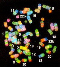 Fig.
3-D from Schröck, E. et al. (1996) Multicolor spectral
karyotyping of human chromosomes. Science
273: 494-497.
Fig.
3-D from Schröck, E. et al. (1996) Multicolor spectral
karyotyping of human chromosomes. Science
273: 494-497.