Goal: To learn how to measure the lengths of chromosome arms
using ImageJ
![]()
VIDEO: See this tutorial in action, then try it yourself,
before going on to the assignment.
0. Save the example files
Hint: It is a good organizational practice to create a folder
to contain all files related to a task eg. you might call it
"example".


| To minimize error in the calibration, it is
better to calibrate using a longer distance, in this case,
the distance between two major tick marks. Draw a line
between the two tick marks. You will note that the line shown begins at the left edge of one tick mark, and ends at the left edge of the adjacent tick mark. Also, the line has to be drawn slightly off of level, since this image is slightly rotated, relative to the horizontal. |
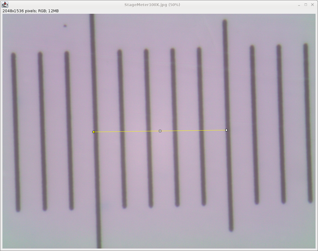 |
| Choose Analyze --> Set Scale. The distance in pixels for the line shown in the example is 868 pixels. Set Known distance to 50, and Unit of length to uM. (For simplicity, we're using "u" to stand for the Greek letter mu.) Also, click on the box that says "Global". This will cause ImageJ to use to calculate lengths in microns, based on the length in pixels, for all images analyzed until you quit ImageJ. |
 |
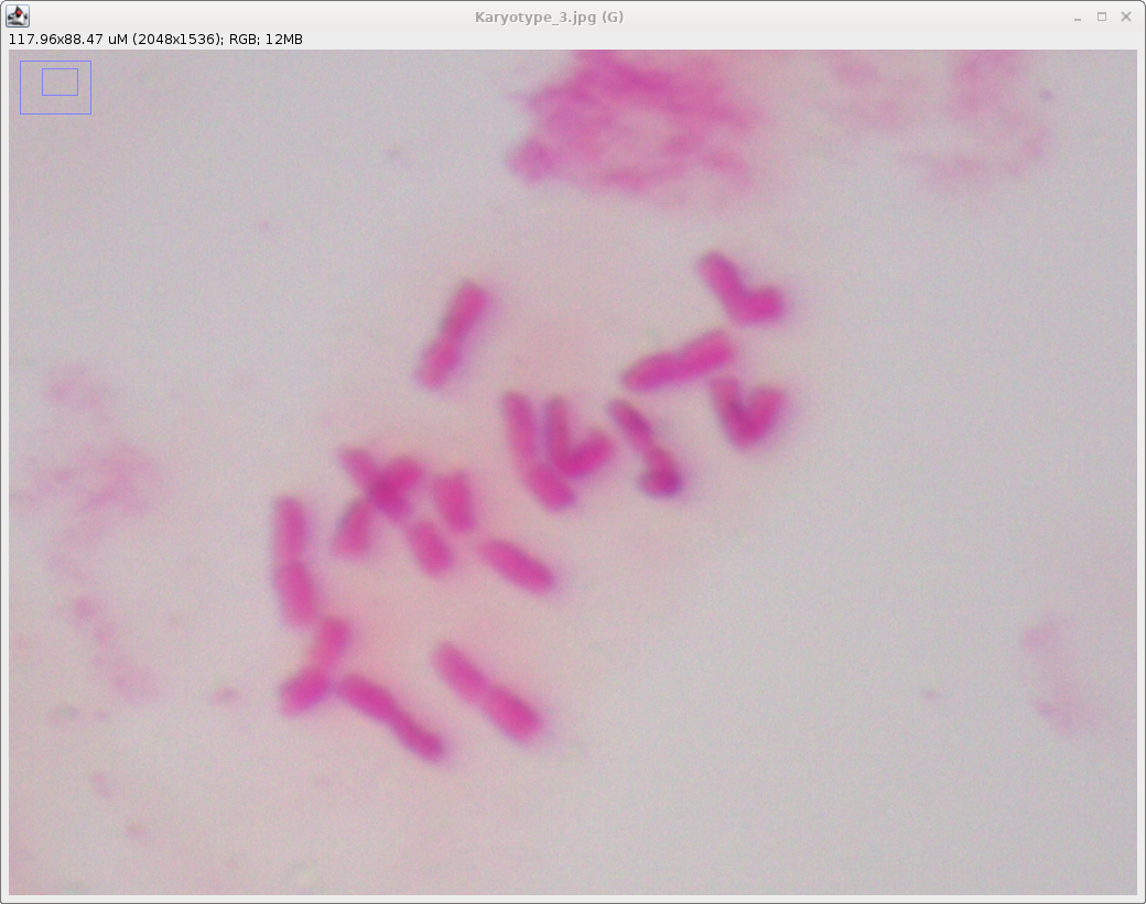
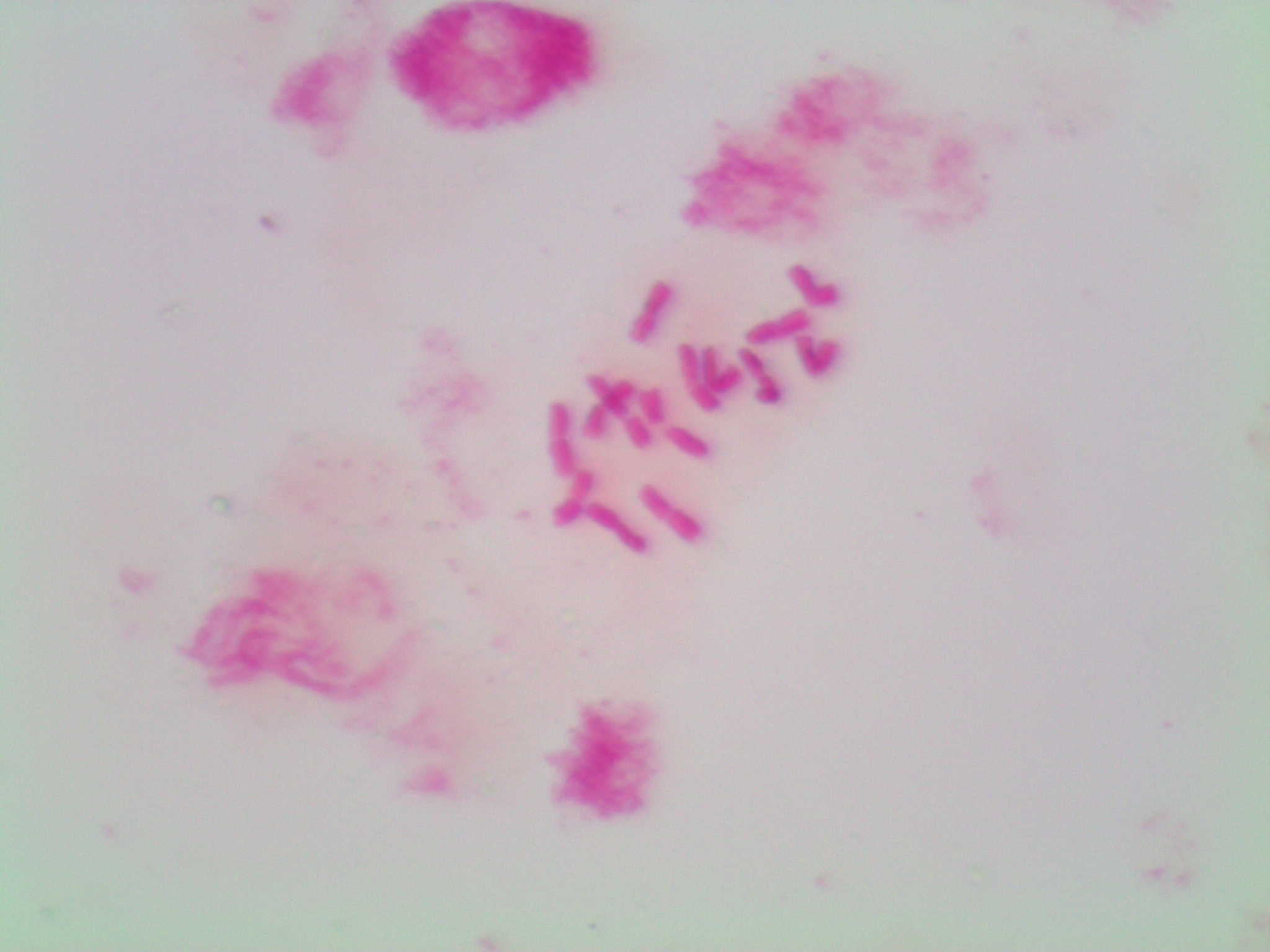
Next, choose File --> Open and
import the file Karyotype_3.jpg. It will be easier to
discern chromosomal features, and to draw measuring lines,
if we zoom in. Click on the zoom tool  , and then click on the image, probably twice.
Use the scrolling tool (hand) , and then click on the image, probably twice.
Use the scrolling tool (hand)  to re-center the image to re-center the image |
 |
| IMPORTANT: ImageJ works
in layers To understand how ImageJ works, you need to understand the concept of layers. Most bitmap graphics programs conceptualize the image as a stack of layers. The first is the raw image itself. If we want to add things, such as labeling, lines or other annotation, we create a separate layer called the Overlay. If you think of the overlay as a transparent sheet that you can lay over a paper photograph, you have the idea. We can draw on the transparent sheet, but never change the photograph below. If we look at the photo through the transparency, we see an annotated picture. We will next show how to create lines for measurement, and add them one by one to the overlay. At the end, we'll save the composite image as a new graphics file. Selection - ImageJ uses the term "selection" to refer to the last object drawn. The selection is temporary, unless you add it to the overlay by clicking ctrl-B, as we'll describe below. It's important to know this term, because it is used extensively in ImageJ documentation. |
| Before we begin, we need to set a few
parameters for the Overlay layer. Choose Image -->
Overlay --> Labels. Make sure the "Show labels" and "Draw backgrounds" boxes are checked. Also, to set Font size to 14. |
 |
| Let's start by drawing lines for the long and short arms of one of the chromosomes. This is done using the Segmented Line tool. Right click on the Line tool and check the box for Segmented line. This tool lets you draw lines with 2 or more segments, which will be critical for measuring chromosomes that have curvature. | 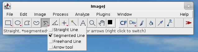 |
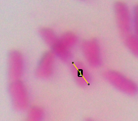
| Let's do the first one, short arm first, then
the long arm. Click the crosshairs at one end of the short
arm, drag along the length, and double click at the
kinetochore. This will leave a yellow line on the short arm. To record the length of this arm, type ctrl-M ( on Mac ⌘-M). The measurement will pop up in the Results window. Because we calibrated using the StageMeter, the Length is in units of µM. Finally, click ctrl-B ( ⌘-B on Mac) to add this arm to the Overlay. |
 |
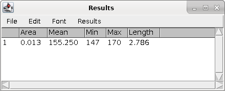 |
| Hint: If you don't like the
line you've drawn, simply draw another line elsewhere. Until
you add a line to the Overlay, it goes away as soon as you
draw something else. Similarly, if you mistakenly add a line
to the results, you can cut that line in the Results box. |
| Again, add the line to the Results box using ctrl-M (⌘-M). Add it to the Overlay using ctrl-B (⌘-B). | 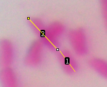 |
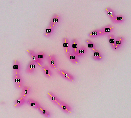
| The final image should look something like
this: One thing to observe is that the chromosome with arms 13 and 14 appears to be overlapped by the chromosome with arm 1 and 2. For the former, it was not entirely clear where the kinetochore was, so these measurements may not be accurate. Also note that for arm 13 and arm 22, it was necessary to draw a segmented line. That means that you click to begin the line, and click as many times as necessary to trace the shape of the arm. The line is completed by double-clicking. |
 |
| This is a common problem, but ImageJ makes it
harder to fix than it should be. Most other programs would
let you simply select the object and "cut" or "delete".
ImageJ makes it more complicated. As an example, you can see that object 5 is a segmented line that incorrectly covers arms from two different chromosomes. We want to delete this object. |
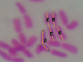 |
| The first step is to get all of the objects
into the ROI Manager. (ROI stands for "Region Of Interest").
Make sure nothing is selected, and choose Image -->
Overlay --> To ROI Manager. This will send all
objects in the overlay into the ROI. In the ROI Manager, click on 0005-0771, which stands for object 5. Object 5 will be highlighted in blue in the image as shown at right. |
 |
| Click the Delete button to delete
object 5. The line will disapear from the list, and from the
image. |
 |
| Click on "Save as Overlay" to save the
changes. |
 |
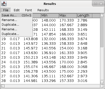
| Also, make sure to save the results as
Results.csv. The .csv file extension indicates that this is a comma-separated value file. CSV is a generic spreadsheet format that can be read or written by any spreadsheet program. In CSV, every line is a row, and on each line, the data items for each column are separated by commas (,). |
 |
| Open Results.csv in your spreadsheet program
(eg. LibreOffice Calc, Excell). If asked about a seperator,
check the Comma box. |
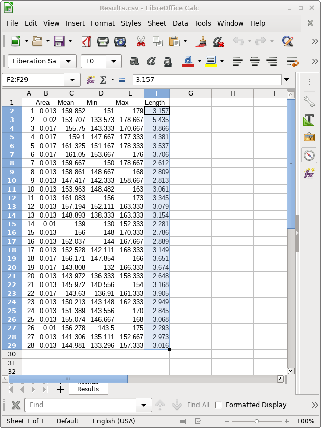 |
| Simply copy the 28 lengths from Results.csv
into column B of the template. The spreadsheet will
automatically calculate long/short arm ratios, and lengths
for the entire chromosome. Save your spreadsheet under a new name eg. karyotype.results.ods. |
 |
If your don't understand how to do something, call me or stop by
my office, or send me a message
at frist@cc.umanitoba.ca. Also,
remember that you can read documentation for each program using
links from the tutorials.