Lecture 4, part 2 of 2
| PLNT4610/PLNT7690
Bioinformatics Lecture 4, part 2 of 2 |
| A |
A |
C |
T |
G |
T |
T |
|
| A |
1 |
||||||
| A |
2 |
||||||
| C |
3 |
||||||
| T |
4 |
||||||
| G |
5 |
||||||
| T |
6 |
||||||
| T |
7 |
Sequence alignment methods predate dot-matrix searches, and all of the alignment methods in use today are related to the original method of Needleman and Wunsch (1970). Needleman and Wunsch wanted to quantify the similarity between two sequences. Over the course of evolution, some positions undergo base or amino acid substitutions, and bases or amino acids can be inserted or deleted. Any measurement of similarity must therefore be done with respect to the best possible alignment between two sequences. Because insertion/deletion events are rare compared to base substitutions, it makes sense to penalize gaps more heavily than mismatches when calculating a similarity score. As an example, a very simple scoring scheme would add +1 for each match, -1 for each mismatch, and -2 for each gap inserted. That is, the larger the gap, the more we subtract. The similarity between two sequences would then be
Similarity = +1(# identities) -1(#mismatches) -2(#gaps)For example:
GCTGGAACCAGSimilarity = 1(8) - 1(2) -2(1) = 4
||||| |||
ACTGGAT-CAG
By definition, the alignment which gives the higest similarity score is the optimal alignment. However, the number of alignments that must be checked increases exponentially with the lengths of the sequences. Allowing gaps also results in an exponential increase in the computation time required.
Although the problem may seem intractably large for all but very small sequences, Needleman and Wunsch conceptualized alignment as a problem in dynamic programming, in which the solution to a large problem is simplified if we first know the solution to a smaller problem that is a subset of the larger problem. Think of an alignment occurring in a matrix, where sequence s of length m is written on the Y-axis, and sequence t of length n is written on the X-axis. The alignment can then be acomplished in two steps:
1. All possible alignments of s and t are contained in array a[0..m,0..n] (the component a[0,0] represents a gap at the beginnning of each sequence).
2. The optimal alignment will be the path through the array that has the highest score, ie. the largest number of matches and fewest mismatches and gaps.
Needleman and Wunch realized that all parts of the alignment problem boiled down to the same decision made at every position i in sequence s, when compared with every position j in sequence t.
If we want to calculate the score at any position a[i,j] in the alignment matrix a, we only have to look at three adjacent cells in the matrix to calculate that score, a[i,j-1], a[i-1,j-1], or a[i-1,j]. These are the positions in the alignment that represent the part of the alignment just prior to a[i,j], at which point either:
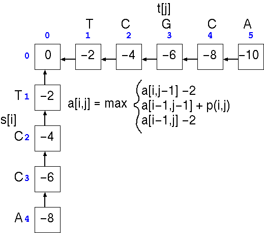
The first step is the
trivial calculation of the case in which one or more terminal
gaps are added to the beginning of either sequence. This is done
by running across the top of the array and progressively adding
a gap penalty (eg. -2) to the score in each cell, and doing the
same to the leftmost column. Next, we apply the three scoring
rules to each cell in the matrix.
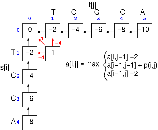
At cell a[1,1], the score is the largest of three possible scores
This process is repeated down the matrix:
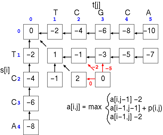
until all cells are filled.
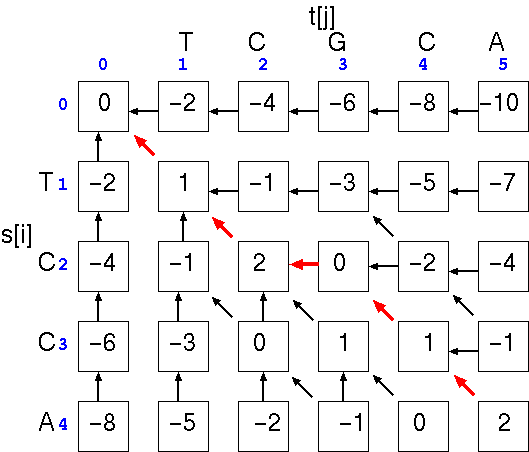
The optimal alignment will be the path that gives the highest total score. In the example, the optimal alignment would be
and the similarity score is simply the score at cell a[i,j], the last cell in the alignment. We can check the score by using the written alignment: 4(+1) + 0(-1) + 1(-2) = 2.TCGCA
|| ||
TC-CA
Note that if we hadn't inserted the gap, the alignment would be
and the similarity score at cell a[i,j], would be: 2(+1) + 2(-1) + 1(-2) = -2. The point is that a single gap can make a large difference in the score.TCGCA
||
TCCA-
Though these examples
give the essence of the Needleman Wunsch method, the literature
contains a wealth of papers improving on this simple algorithm.
| Example of an optimal alignment between cDNA
sequences for defensin genes from Pea (PPEADRR230B) and
Cucumber (CAGT). The alignment was produced by GLSEARCH from the FASTA package. n-w opt: The raw Needleman-Wunch alignment score Z-score: Standard Deviations of the best score relative to the mean of all alignments tested. bits: Measure of information content of the alignment ie. how it differs from a random alignment. E: Probability of seeing an alignment this good by comparing two arbitrary sequences of similar nucleotide content. |
Statistics: (shuffled [500]) Unscaled normal statistics: mu= -90.3780 var=579.7105 Ztrim: 0 |
Forcing the entire
length of both sequences into alignment may not be a realistic
representation of the similarity. In most cases, only a
particular block of nucleotides or amino acids have a compelling
degree of similarity, while flanking regions may not. As well,
considering regions out side the homologous region requires
extra computational space and time, which we recall increases
with the square of the length.
For these reasons Smith
and Waterman developed a modification of the NW algorithm, now
referred to as SW. In essence, when SW encounters a negative
score at any point in the matrix, it sets the score of that x,y
cell to 0. The result of setting this score to 0 is to prevent
the algorithm from trying to extend into regions that would
negatively contribute to the score. The following table
summarizes the differences between NW and SW.
| Smith–Waterman algorithm | Needleman–Wunsch algorithm | |
|---|---|---|
| Initialization | First row and first column are set to 0 | First row and first column are subject to gap penalty |
| Scoring | Negative score is set to 0 | Score can be negative |
| Traceback | Begin with the highest score, end when 0 is encountered | Begin with the cell at the lower right of the matrix, end at top left cell |
from https://en.wikipedia.org/wiki/Smith%E2%80%93Waterman_algorithm
Significance: SW drastically speeds up the NW algorithm by
eliminating flanking regions which cannot possibly improve the
alignment, resulting in a local alignment with the same rigor as
the exhaustive NW algorithm.
penalty = gap_begin + (# gaps * gap_extend)Example: For a 2 base gap in a DNA pairwise alignment, if gap_begin = -10 and gap_extend=-1, the gap penalty is -10 + 2(-1) = -12.
Construction of
biologically significant alignments should take into account the
fact that protein evolution is constrained by the chemical
properties of amino acids, and by the degeneracy of the genetic
code. Chemically conservative replacements tend to occur more
frequently than replacements with amino acids that are
chemically different. For example, it is far more likely to see
a substitution of Leucine with Isoleucine, both of which are
non-polar, than a substitution of Aspartic acid, which is
negatively-charged, for Leucine.
Secondly, the observed
frequencies of substitution will depend on the genetic code.
Amino acid substitutions that require only a single nucleotide
replacement will occur more frequently than substitutions
requiring 2 or 3 nucleotide replacements.
Scoring matrices have been constructed to replace the p(i,j) function above. That is, for any possible amino acid substitution, a value from the scoring matrix is added to the similarity score, rather than adding 1 for an identity and -1 for a mismatch. One of the most commonly-used scoring matrices is the PAM250 matrix, shown below:
Cys 12Substitution of an Aspartic acid for Glutamic acid (both acidic) adds 3 to the score. Substitution of the positively-charged Lys for the non-polar Pro adds -1 to the score. Generally, the more conservative the replacement, the higher the value that will be added to the score.
Gly -3 5
Pro -3 -1 6
Ser 0 1 1 1
Ala -2 1 1 1 2
Thr -2 0 0 1 1 3
Asp -5 1 -1 0 0 0 4
Glu -5 0 -1 0 0 0 3 4
Asn -4 0 -1 1 0 0 2 1 2
Gln -5 -1 0 -1 0 -1 2 2 1 4
His -3 -2 0 -1 -1 -1 1 1 2 3 6
Lys -5 -2 -1 0 -1 0 0 0 1 1 0 5
Arg -4 -3 0 0 -2 -1 -1 -1 0 1 2 3 6
Val -2 -1 -1 -1 0 0 -2 -2 -2 -2 -2 -2 -2 4
Met -5 -3 -2 -2 -1 -1 -3 -2 0 -1 -2 0 0 2 6
Ile -2 -3 -2 -1 -1 0 -2 -2 -2 -2 -2 -2 -2 4 2 5
Leu -6 -4 -3 -3 -2 -2 -4 -3 -3 -2 -2 -3 -3 2 4 2 6
Phe -4 -5 -5 -3 -4 -3 -6 -5 -4 -5 -2 -5 -4 -1 0 1 2 9
Tyr 0 -5 -5 -3 -3 -3 -4 -4 -2 -4 0 -4 -5 -2 -2 -1 -1 7 10
Trp -8 -7 -6 -2 -6 -5 -7 -7 -4 -5 -3 -3 2 -6 -4 -5 -2 0 0 17
Cys Gly Pro Ser Ala Thr Asp Glu Asn Gln His Lys Arg Val Met Ile Leu Phe Tyr Trp
Substitution matrices
like PAM250 are constructed by observing the frequencies of
amino acid replacements in large samples of protein sequences.
For a given replacement, the PAM value is proportional to the
natural log of the frequency with which that replacement was
observed to occur.
The Blosum series of matrices are also commonly-used.
Gly   7
Pro  -2   9
Asp  -1  -1   7
Glu  -2   0   2   6
Asn   0  -2   2   0   6
His  -2  -2   0   0   1  10
Gln  -2  -1   0   2   0   1   6
Lys  -2  -1   0   1   0  -1   1   5
Arg  -2  -2  -1   0   0   0   1   3   7
Ser   0  -1   0   0   1  -1   0  -1  -1   4
Thr  -2  -1  -1  -1   0  -2  -1  -1  -1   2   5
Ala   0  -1  -2  -1  -1  -2  -1  -1  -2   1   0   5
Met  -2  -2  -3  -2  -2   0   0  -1  -1  -2  -1  -1   6
Val  -3  -3  -3  -3  -3  -3  -3  -2  -2  -1   0   0   1   5
Ile  -4  -2  -4  -3  -2  -3  -2  -3  -3  -2  -1  -1   2   3   5
Leu  -3  -3  -3  -2  -3  -2  -2  -3  -2  -3  -1  -1   2   1   2   5
Phe  -3  -3  -4  -3  -2  -2  -4  -3  -2  -2  -1  -2   0   0   0   1   8
Tyr  -3  -3  -2  -2  -2   2  -1  -1  -1  -2  -1  -2   0  -1   0   0   3   8
Trp  -2  -3  -4  -3  -4  -3  -2  -2  -2  -4  -3  -2  -2  -3  -2  -2   1   3  15
Cys  -3  -4  -3  -3  -2  -3  -3  -3  -3  -1  -1  -1  -2  -1  -3  -2  -2  -3  -5  12
     Gly Pro Asp Glu Asn His Gln Lys Arg Ser Thr Ala Met Val Ile Leu Phe Tyr Trp Cys
One criticism of the PAM
matrices is that the PAM units were calibrated using pairs of
closely-related proteins, because these could be aligned by
hand. However, PAM1 units are extrapolated to high PAM values
(eg. PAM250), so it is uncertain how realistic these
extrapolated values are.
The Blosum matrices
were calculated using data from the BLOCKS* database [http://blocks.fhcrc.org ],
which contains alignments of more distantly-related proteins. In
principle, Blosum matrices should be more realistic for
comparing distantly-related proteins because the matrices are
derived from distantly-related proteins. On the other hand, one
could argue that the more distantly related proteins are, the
less reliable the alignment, which could contribute to error in
the calculation of Blosum matrices.
*Note: The
BLOCKS database is no longer supported. This just goes to show
a chronic problem in bioinformatics - the original datasets
used to build empiracally-derived computational tools become
more difficult to find as the original data sinks into
obsolescence.
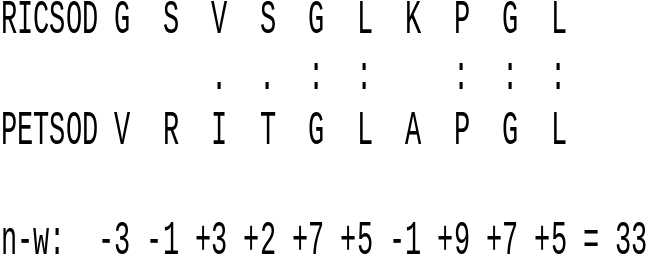
| Example:
Calculation of the Needlwman-Wunsch score for a short
segment of superoxide dismutase proteins from rice and
parsley. The BLOSUM 45 scoring matrix was used. : - identities . - similar amino acids |
|
Equivalent PAM and Blossum matrices

 Unless otherwise cited or
referenced, all content on this page is licensed under
the Creative Commons License Attribution
Share-Alike 2.5 Canada Unless otherwise cited or
referenced, all content on this page is licensed under
the Creative Commons License Attribution
Share-Alike 2.5 Canada |
| PLNT4610/PLNT7690
Bioinformatics Lecture 4, part 2 of 2 |