Lecture 10, part 1 of 2
| PLNT4610/PLNT7690
Bioinformatics Lecture 10, part 1 of 2 |
To understand the problem of genomic sequencing, we need to
understand the properties of prokaryotic and eukaryotic genomes
| Prokaryotes |
Eukaryotes |
|
| taxa |
bacteria,
archaea |
fungi,
protists, plants, animals |
| genome structure |
single
circular chromosome plasmids |
two
or more linear chromosomes circular organelle genomes: mitochondrial, plastid |
| ploidy levels |
haploid |
diploid,
tetraploid, hexaploid or higher |
| total genome length (bp) |
106
- 107 |
107 - 1012 |
| complexity |
single
copy |
|
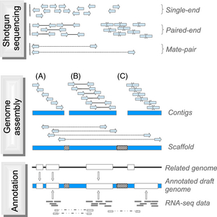
As sequencing technologies have given longer reads,
combined with paired-end reads, it has been possible to assemble
complete prokaryotic genomes by the whole genome shotgun approach.
However, the complexity of most eukaryotic genomes makes it almost
impossible to get complete genomic sequences at today's
level of technology.
The first complete genomic sequences for eukaryotes were done using a "divide and conquer" strategy.
1. Construct a representative BAC library (avg. insert ~ 100 kb)
2. For each chromosome, find a set of overlapping BAC clones whose
inserts cover the entire chromosome. In this way, the location of
each BAC on the chromosome is known.
3. Sequence each BAC separately using shotgun sequencing.
| Summary of Whole Genome Sequencing |
 |
| Platform |
Read length |
Reads/unit |
Read Type |
Error type |
Comment |
| Illumina |
200 - 600 |
10 - 375 million |
PE, SR |
substitution |
highest throughput |
| Ion Torrent |
200 - 400 |
0.4 - 60 million |
SR |
homopolymers |
|
| Pac Bio |
4600 - 14,000 |
22,000 - 47,000 |
SR |
indel |
longest reads highest error rate |
| Oxford nanopore |
15,000 - 20,000 |
|
SR |
homopolymers; deletions |
longest reads can exceed 1000 kb |
| Roche 454 |
400 - 700 |
20,000 - 350,000 |
SR |
indel |
lowest error rate |
| SR - single
read; PE - paired end |
|||||
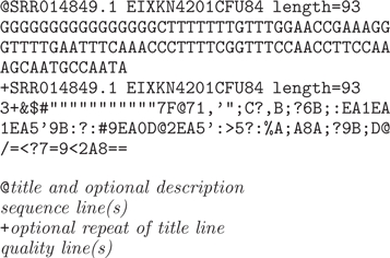
| Definition of Fastq format for sequencing
reads The information for each read consists of four lines per read. line 1 - unique identifier of read line 2 - sequence of read line 3 - either '+' or optional repeat of title line 4 - quality of each base read. (Note: 4 lines are shown at right, but the sequence lines are long, so they wrap.) |
 |
||||||||||||||||||||||||||||||||||||||||
| Quality encoding Phred quality scores are typically calculated as Q = -10 x log10(Pe) where Pe is the estimated probability of error. To save space in fastq files, Q values are encoded as single ASCII characters whose values, such that the Q value is represented by the ASCII character whose decimal number plus some offset value, usually 33 or 64. For example, in a Q value of 34 is encoded by the number in the ASCII character chart with the decimal value 33 + 34 = 67 ie. the capital C. A Q value of 30, plus offset 33, gives the ASCII decimal value of 63, represented by the ASCII character question mark (?). Note: Some sequence assembly programs need to know which offset your data uses, 33 or 64. |
|
||||||||||||||||||||||||||||||||||||||||
| The first step after receiving sequencing
read files should be to look at the quality of the reads
using FastQC,
which creates reports of the overall quality of the
sequencing results. The example shown below is for a good
sequencing run, in which the quality of the nucleotide calls
is in the high range at all positions. For positions
approaching 145 nt, the variation in quality of the reads
gets larger. For this data, it is probably best not to use
positions above 145 - 149 for sequence assembly. Most
assembly programs will automatically filter out poor quality
positions.
|
|

| Keep in mind: When you trim reads from fastq files, you generate new fastq files that are almost the same size as the original files. Thus, if you have sequencing read files totaling to 25 Gb, after trimming there will be an additional 25 Gb of fastq files with the trimmed reads. As well, the next step is error correction, which would generate another 25 Gb of trimmed, corrected reads. A good rule of thumb therefore is that for a genome sequencing project you need more than 3x the disk space required for the original raw reads. |
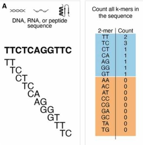
| Any sequence can be thought of as a nested
set of k-mers. K-mer tables are a hash (dictionary) of all
k-mers in the sequence, and their counts. The trivial example shows a k-mer table for the trivial case of k=2. For k=2, there are 42 = 16 possible k-mers. Typical k-mer tables are made for k-mers of 21 nucleotides or larger. Usually only a fraction of the possible k-mers are found in the sequence (blue). k-mers missing from the genome (orange) are referred to as "nullomers". Hash tables are data structures that are highly efficient to search. |
 from Moeckel C et al. (2024) A survey of k-mer methods and applications in bioinformatics. Computational and Structural Biotechnology Journal 23:2289-2303. DOI: 10.1016/j.csbj.2024.05.025. |
"For sufficiently large k, almost all single-base errors alter k-mers overlapping the error to versions that do not exist in the genome. Therefore, k-mers with low coverage, particularly those occurring just once or twice, usually represent sequencing errors. For the purpose of our discussion, we will refer to high coverage k-mers as trusted, because they are highly likely to occur in the genome, and low coverage k-mers as untrusted. Based on this principle, we can identify reads containing untrusted k-mers and either correct them so that all k-mers are trusted or simply discard them."Put another way, k-mers that are real should occur in all reads mapping to a particular site in the genome, while erroneous k-mers might be found only once in a dataset.
| k |
4k |
Max. genome size (Mb)
cutoff (4k/200) for this k-value |
example species |
Genome size (Mb) |
| 15 |
1.07e9 |
5.37 |
Escherichia coli |
5.43 |
| 16 |
4.2e9 |
21.5 |
Saccharomyces cereviseae |
12.12 |
| 17 |
1.7e10 |
85.9 |
Leptosphaeria maculans |
45.12 |
| 18 |
6.87e10 |
344 |
Drosophila melanogaster |
143.7 |
| 19 |
2.75e11 |
1374 |
Solanum tuberosum |
705.9 |
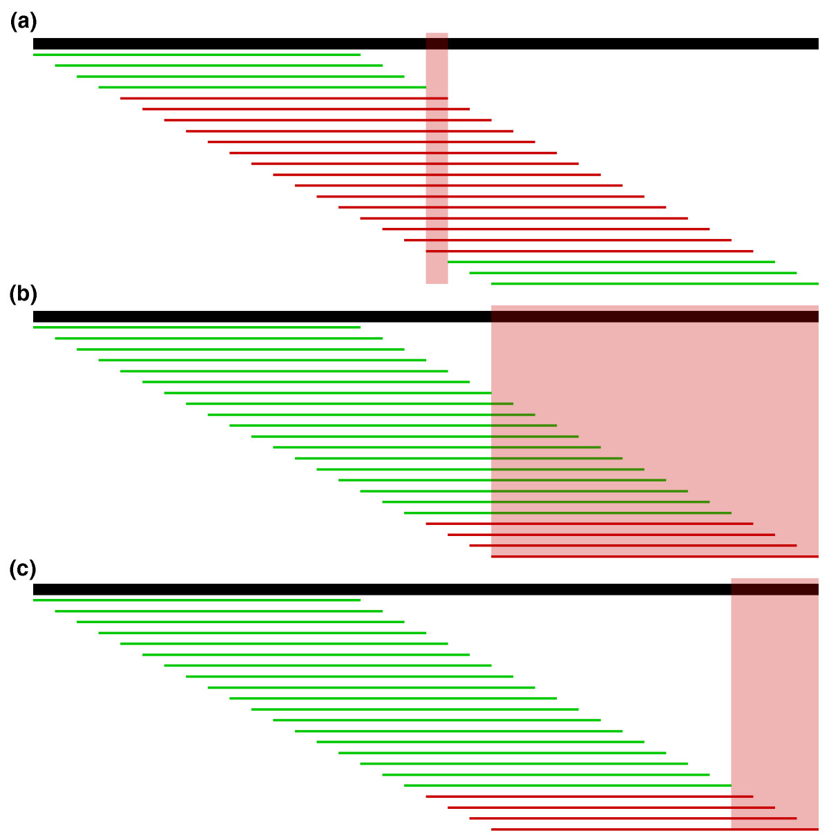
| Localize errors. Trusted (green) and
untrusted (red) 15-mers are drawn against a 36 bp read. In
(a), the intersection of the untrusted k-mers localizes the
sequencing error to the highlighted column. In (b), the
untrusted k-mers reach the edge of the read, so we must
consider the bases at the edge in addition to the
intersection of the untrusted k-mers. However, in most
cases, we can further localize the error by considering all
bases covered by the right-most trusted k-mer to be correct
and removing them from the error region as shown in (c). Fig. 4 from Kelly et al. To correct errors, untrusted k-mers are replaced by trusted k-mers that could correct the error. The most likely corrections are tried, based on quality information, until a set of corrections is found that makes all k-mers in a read into trusted k-mers. |
 |
| # encode all
k-mers from all reads into table for each read do trim N's from ends of read replace internal N's with an arbitrary nucleotide add all k-mers from read to k-mer table # Get rid of any k-mer that is only represented once for each k-mers in table if count(k-mer) = 1 remove k-mer from table for each read do find all potential error positions as localized drop in k-mer frequency for each error position try correcting by insertions, deletions, substitutions choose best correction if valid(correction) apply(correction to read) else # assume homopolymer correction try different lengths of homopolymer choose best correction if valid(correction) apply correction to read A more complete pseudo-code for the algorithm is found in the Marnier et al. publications |
| nucleotide |
binary representation |
| A |
00 |
| G |
01 |
| C |
10 |
| T |
11 |

 Unless otherwise cited or
referenced, all content on this page is licensed under
the Creative Commons License Attribution
Share-Alike 2.5 Canada Unless otherwise cited or
referenced, all content on this page is licensed under
the Creative Commons License Attribution
Share-Alike 2.5 Canada |
| PLNT4610/PLNT7690
Bioinformatics Lecture 10, part 1 of 2 |