• Corn Genetics
• Monohybrid Cross
• Statistical Evaluation of the Results

Corn Genetics

Many models are useful for illustrating basic Mendelian genetics. Whether you use the fruit fly, corn, sweet pea or some other system the basic principles are applicable to all diploid systems including humans. We will be using corn to illustrate some of these principles. Mature corn plants produce ears that contain hundreds of seeds or kernels. Each seed is formed by the fertilization of an egg by a male gamete. Therefore, each kernel on an ear of corn can grow into a whole new plant. A complete ear represents a compact population of offspring which may be sampled.

Corn cob showing many individuals (each was produced by a single egg and sperm)

  Monohybrid Cross

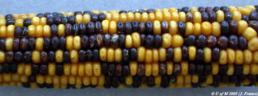
The cob bears fruit (the seeds) which are either purple or yellow in color. The color of the corn fruit is inherited in exactly the same way as the color of the flowers on Mendel's peas. The cob above was taken from a corn plant which was a F₂ plant resulting from an original parental cross between a homozygous purple fruit plant and a homozygous yellow fruit plant. The allele A (purple) is dominant over the recessive allele a (yellow).

Examine the cob above and answer the following questions:

• What proportion of the fruit on this cob do you expect from theory to be purple?
• What proportion do you expect to be yellow?

Click here for a diagramatic representation of a monohybrid cross using corn

Using more than 5 rows of fruits, count 100 fruits and record your results:

Purple

Yellow

Total 100

• Do these results agree with the proportions you expected?

  Statistical Evaluation of the Results

If you flip an "honest" coin 10 times you may predict that you would get 5 heads and 5 tails, however in actuality you may obtain results which are quite different from the predicted, perhaps 6-4, 7-3, etc. Biologists frequently deal with observations (data) which deviate from the expected or predicted. The question then is whether or not the deviations observed between actual data and predictions are what you would expect by chance alone or whether other factors are involved. If the deviation from expected can not be explained by chance then perhaps the prediction is incorrect. Statistics allows the researcher, through mathematical examination of the data, to determine how closely the data fits predicted expectations, and whether or not deviation can be explained by chance.

Two important factors to consider in statistics are sample size and the way in which the sample is obtained. Obviously if you flip the coin just twice as compared to say 1000 times one might expect dramatically different proportions of heads and tails. If you made inferences about the entire population based on a sample of two you may come to some rather extreme conclusions. Not only must the sample be of sufficient size to accurately reflect the total population it must also be obtained in a random fashion.

We will be using the Chi-Square Test to see whether the data you have obtained from the monohybrid cross involving purple and yellow corn kernels fits your predicted values. The Chi-Square test is a statistical test frequently used to see whether data obtained in a genetic cross fits a predicted ratio. The formula for Chi-Square is:

d = deviation from the expected

e = expected value

 

Use the data that you obtained by counting 100 kernels of corn to complete the following table:

Sum the final two cells to determine your chi-Square value.

• Was the sample a random sample?
• Can you think of a way to count to insure a random sample?

You can also use the following to calculate your value. However, you must understand how the calculation is made for examination purposes.

 CHI-SQUARE CALCULATOR
 

Enter the observed number and the expected ratio below.

Observed #

Ratio

CATEGORY 1 
CATEGORY 2 
CATEGORY 3 
CATEGORY 4 

Observed
Expected
chi-square

 

Interpretation of CHI-SQUARE

The value is then used to determine how good a fit there is between the observed values and the expected values. If you have an exact fit (i.e. the observed is the same as the expected) the value of will be zero and the greater the deviation between the observed and the expected the larger will be the value of . The value of indicates the degree of discrepancy from the expected. The question then is how do we determine if the value is large enough to suggest that the hypothesis is incorrect (i.e. you have the wrong explanation to arrive at the expected results)? To do this you must compare your value to a table of values. To use the table you need to know one more parameter, the degrees of freedom. The degrees of freedom is numerically equal to the number of classes minus one. In our case there are only two classes (purple and yellow) and therefore the degrees of freedom is one (2-1).

• If you were using the results of the F₂ of a dihybrid cross for calculating a how many degrees of freedom would you use?

Evaluation of the Results:

Examine the table of values below. Note the value 3.84 in the column under p = 0.05 and corresponding to one degree of freedom. The table states that for one degree of freedom that a of 3.84 has a chance probability of 0.05 (5%), in other words deviation from expected as great as 3.84 will occur by chance alone in about one in 20 trials. If your calculated is less than 3.84 (quite likely it will be) this would mean that the deviation observed in the experiment can be expected by chance alone even more often than once in 20 trials. Another way of stating this is that with a of 3.84 or less there is no significant difference between your expected results and your experimental results so in our case we would say that yes that is a 3:1 cob. The difference you see is what you could reasonably expect by normal chance fluctuations. By convention most biologists accept deviations having a chance probability as great as or greater than 0.05 (1 in 20) as not being statistically significant. If on the other hand your calculated was greater than 3.84 then you might argue that the variation was greater than you would expect by chance alone and perhaps the hypothesis was incorrect or there was some error in the way the data was gathered.

 

First published Sept 95: Modified June 2019
Copyright © Michael Shaw 2019 (Images and Text)

Return to Biology Home Back to Lab Index Forward to Next Page University of Manitoba Home