| The PHYLIP programs are command line
programs, but can
be run by GDE The programs in the PHYLIP package are interactive programs designed to be run at the command line. GDE can run these programs by generating the keystrokes needed to set programs parameters. |
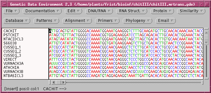
Create a directory called parsimony, and save chitIII.mrtrans.gde
to this directory. Open the file in GDE:
OUTFILE - the
report on the phylogeny
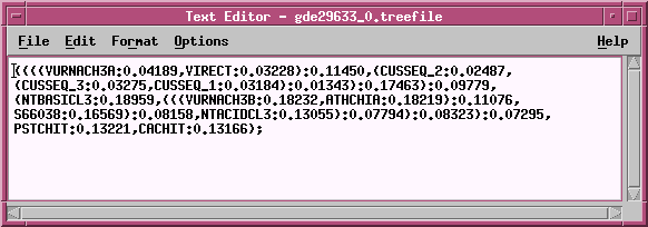
TREEFILE -
the machine -readable treefile. Readable by
programs such as DRAWTREE, DRAWGRAM, and TREETOOL.
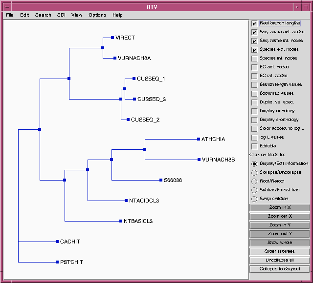
ATV - the treefile in the ATV tree editor.
Parsimony methods set out to build a tree by successively adding sequences to the tree, until all sequences have been added. Unlike distance methods, which tend towards a single answer, the tree you get could be strongly influenced by the order in which branches are added.
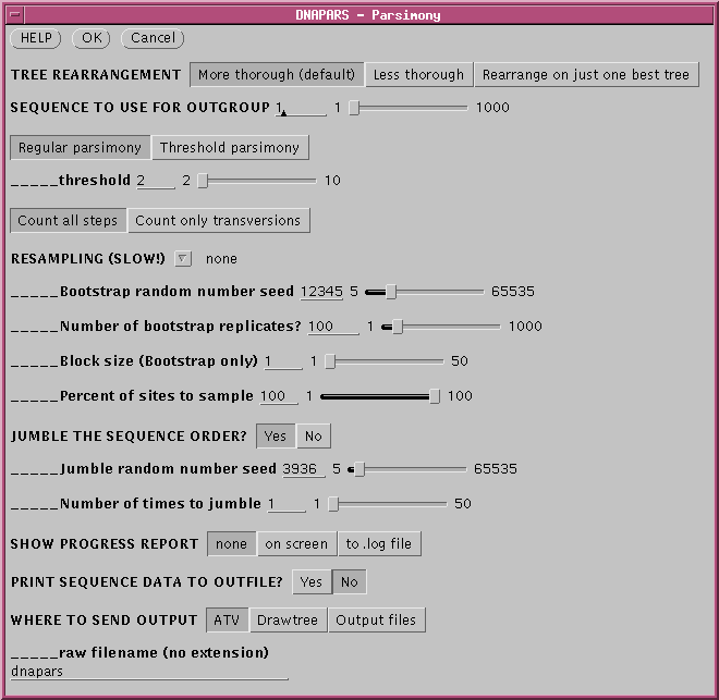
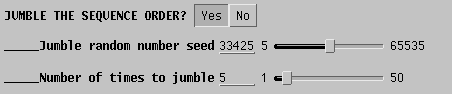
To randomize the order of sequence addition, choose 'Yes' in the
Jumble
area of the DNAPARS menu, and set a random number using the slider, to
seed the random number list. Usually only a few jumbles are needed to
uncover
most of the alternate trees. In the example, the search is repeated 5
times
with a random order of sequences.
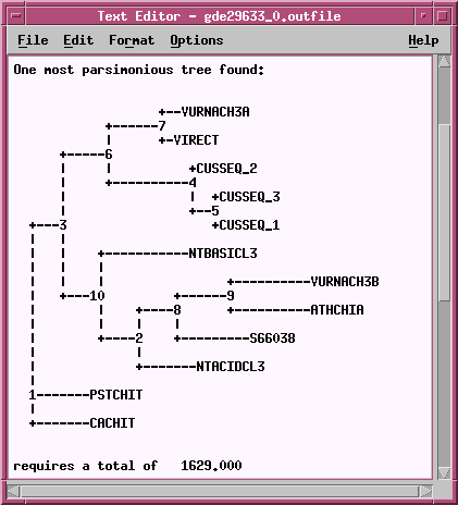
Two equally parsimonious trees are produced.
+--VURNACH3B |
+--VURNACH3A |
Many of the groups of sequences cluster together in both trees. However, sequences shown in bold on the tree (NTACIDCL3, ATHCHIA, VURNACH3B, NTBASICL3, S66038) cluster together in the tree at right, but are split among several clades in the tree at left. The fundamental topology of the tree is therefore dependent upon the order in which the sequences are added.
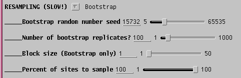
By default, 100 bootstrap replicate datasets will be created, each containing positions sampled at random from the sequence alignment . In each set, some positions will be overrepresented, and others underrepresented. A large enough set of replicates should ensure that all parts of the sequence are equally biased among the replicates as a whole. If the original tree was simply due to a fortuitous circumstance that a few positions tipped the balance between one topology and another, different topologies will appear as each replicate dataset is evaluated. If the data are robust, meaning that a given branch appears regardless of which sites are omitted from the sample, then that branch is strongly supported by the data.
Since 100 bootstraps require 100 iterations of the tree buiilding
process,
the time required can be substantial when there are large numbers of
sequences.
It is therefore a good practice to send output to files, rather than to
windows:
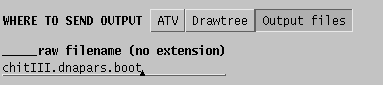
In this case two files will be created:
chitIII.dnapars.boot.outfileThe trees created during the 100 runs of DNAPARS are combined into a consensus tree, showing the number of times each branch occurred amont 100 bootstrap replicates.
chitIII.dnapars.boot.treefile
+------------------------------------------------VIRECT |
From the two parsimony trees examined above, we got a rough idea of which groups should cluster together. For example, CUSSEQ1, 2 & 3 should all cluster together, although surprisingly, CUSSEQ3 clusters with CUSSEQ1 in 61% of the trees, this is not true in 39% of the trees. The least certain grouping in the tree is the clustering of NTBASICL3, ATHCHIA, VURNACH3B and NTACIDCL3. These only cluster together 32% of the time.
Bootstrapping therefore gives us a way to determine which parts of
the
tree are most strongly supported by the data, and which are not.
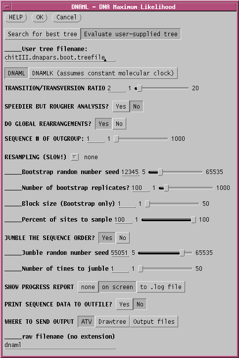
In this example, "Evaluate user-supplied tree" is chosen, and "chitIII.dnapars.boot.treefile" is chosen as the treefile to use.
The contents of the output file (chitIII.dnaml.outfile)
are shown below. The machine-readable tree is in chitIII.dnaml.treefile.
DNAML
JUMBLING SEQUENCE ORDER 1 ITERATIONS, SEED=55049
Nucleic acid sequence Maximum Likelihood method, version 3.63
Empirical Base Frequencies:
A 0.25559
C 0.24475
G 0.23579
T(U) 0.26388
Transition/transversion ratio = 2.000000
User-defined tree:
+--------PSTCHIT
|
| +--VURNACH3A
| +------1
| | +-VIRECT
| +----2
| | | +--CUSSEQ_1
| | | +--4
| | +----------------3 +--CUSSEQ_3
| | |
| | +-CUSSEQ_2
10---5
| | +-------------------NTBASICL3
| | +--8
| | | | +-------------VURNACH3B
| | +---7 +-----9
| | | | +--------------ATHCHIA
| +----6 |
| | +------------NTACIDCL3
| |
| +--------------S66038
|
+----------CACHIT
remember: this is an unrooted tree!
Ln Likelihood = -7100.58654
Between And Length Approx. Confidence Limits
------- --- ------ ------- ---------- ------
10 CACHIT 0.18428 ( 0.14362, 0.22496) **
10 PSTCHIT 0.15332 ( 0.11580, 0.19088) **
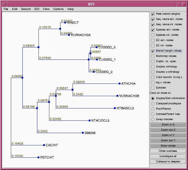
10 5 0.06367 ( 0.03189, 0.09550) **
5 2 0.08925 ( 0.05357, 0.12493) **
2 1 0.12015 ( 0.08333, 0.15697) **
1 VURNACH3A 0.04962 ( 0.03107, 0.06823) **
1 VIRECT 0.02927 ( 0.01360, 0.04493) **
2 3 0.27939 ( 0.22660, 0.33224) **
3 4 0.00857 ( zero, 0.01907) *
4 CUSSEQ_1 0.03580 ( 0.02140, 0.05029) **
4 CUSSEQ_3 0.03501 ( 0.02064, 0.04935) **
3 CUSSEQ_2 0.02707 ( 0.01328, 0.04087) **
5 6 0.08199 ( 0.04707, 0.11699) **
6 7 0.06701 ( 0.03375, 0.10031) **
7 8 0.03705 ( 0.00901, 0.06509) **
8 NTBASICL3 0.32805 ( 0.26705, 0.38904) **
8 9 0.09247 ( 0.05329, 0.13174) **
9 VURNACH3B 0.24920 ( 0.19734, 0.30108) **
9 ATHCHIA 0.26028 ( 0.20748, 0.31311) **
7 NTACIDCL3 0.22492 ( 0.17728, 0.27257) **
6 S66038 0.25430 ( 0.20315, 0.30545) **
* = significantly positive, P < 0.05
** = significantly positive, P < 0.01
Execution times on smith: 2.0u 0.0s 0:02 88% 0+0k 0+0io 0pf+0w
| WARNING
Maximum likelihood methods are very slow, because they attempt to consider an enormous number of possible trees. The time required increases exponentially with the number of sequences. Therefore doubling the number of sequences does not double the execution time. In fact for DNAML, the time required increases roughly with thr 4th power of the number of the sequences! For most practical purposes, direct tree construction with greater than 30 sequences requires prohibitive amounts of time. Since bootstrapping multiplies the time required often by a
factor of
100 or more, we usually don't have the luxury of bootstrapping with
maximum
likelihood methods. However, as illustrated above, we can bootstrap
with
a less time consuming method such ase parsimony, and then build the
final
tree with Maximum Likelihood. |
Note that the original tree had a log likelihood of -7100.58644. After trying global rearrangements of this tree, in which 306 alternative trees were tested, a slightly different tree with a log likelihood of -7094.81002 was found. The difference in likelihoods between these two trees is roughly -7101 - (-7095) = -6. Recalling that these are logs to the base e, e6 = 403. Therefore the final tree is 403 times more likely to produce the data than the original tree.
A note on execution times - The execution time shown in the
example
is not the time that fastDNAml would require to build this tree from
scratch.
It is simply the time required to evaluate the tree it was given, doing
some rearrangements, but leaving most of the tree intact. When the tree
was built from scratch using DNAML, the execution times were:
Execution times on smith: 152.0u 0.0s 2:33 99% 0+0k 0+0io 0pf+0w
Therefore, a de-novo construction of this tree would require 152 seconds of CPU time, and took 2 minutes 33 seconds elapsed time.