CGH File Loader
The scripting capabilities within MeV permit the execution of multiple algorithms to be performed without user oversight or intervention once processing begins. The execution steps are dictated by a user-defined script that describes the parameters to use for the selected algorithms. Scripting in MeV allows one to document the algorithms run and the selected parameters during data analysis. The script document can be shared with collaborators so that analysis steps can be replicated on the common data set. Scripting is also useful when running several long analysis steps that would normally require monitoring in MeV's interactive mode. Each algorithm and the parameters are pre-selected in the script so the next algorithm kicks off as soon as the previous run finishes. Despite the advantages of scripting, there may be times when careful evaluation of a result before deciding on the next algorithms is needed. In this setting scripting might be used as a first pass analysis and the multiple results of the script run can lead to the selection of different algorithms or new parameter selections.
Currently CGH Analyzer is capable of loading experiments only in one generic format. We will provide other loaders to accommodate various other formats in the future. Currently CGH Viewer supports only 2 species data: Human & Mouse.
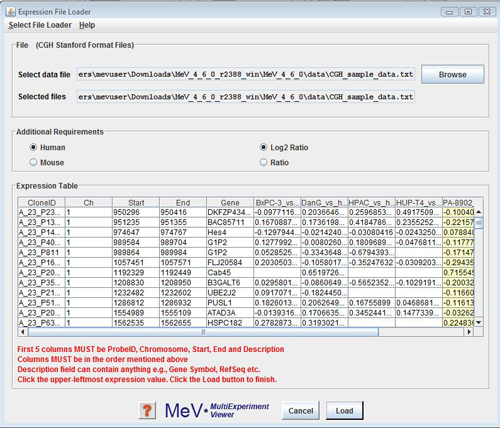
CGH Analyzer allows data to be loaded from one format only. The format includes 4 mandatory columns followed by sample columns. The mandatory columns are:
The mandatory columns are followed by Sample observations where each observation for each probe is the log2 or simple intensity ratio of Cy3 & Cy5. If the observations are not log2 transformed they are done so by the module.
The protocol for loading data from files is as follows:
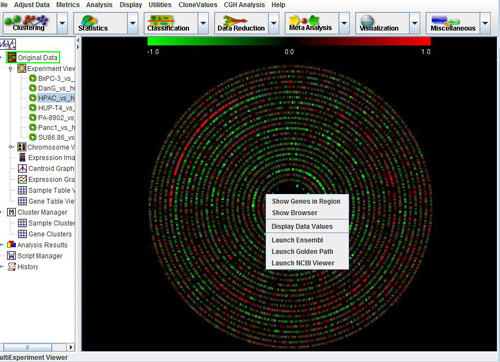
Once experiments have been loaded, the Main View node of the navigation tree should contain a subtree called Experiment Views. Expand this subtree to display a list of all the samples that have been loaded. Clicking on any of these samples will display the CGH Circle Viewer for that sample.
The CGH Circle Viewer is a circular representation of the entire genome of a sample. This view provides easy identification of large scale abnormalities and overall aneuploidy of a sample. The display consists of 24 concentric circles, each representing a chromosome, with chromosome 1 represented by the outermost circle and chromosome Y represented by the innermost circle. Each circle is composed of a series of colored dots, each representing a probe. The probes are arranged by their linear around the genome. The p-arm of each chromosome begins at 180 degrees from the center of the display and subsequent probes are arranged clockwise by their position on the chromosome.
Click on any clone in the circle viewer to display its clone name and chromosome. Right Clicking on any region will display a menu to browse RefSeq genes in the region, Launch CGH browser on a sample, Map out to public domain sites like NCBI, etc.
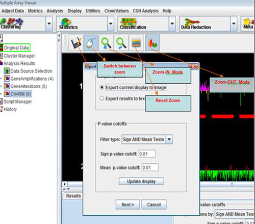
The CGH Analyzer currently allows one method of determining the value for each probe, i.e. the log2 ratio. All displays by default are a red/green ratio gradient color display. Each element is red, green, black or gray. Black elements have a log average inverted ratio of 0, while green elements have a log ratio of less than 0 and red elements have a log ratio greater than 0. The further the ratio from 0, the brighter the element is. Gray elements are missing or were determined as bad by the spot quality filtration criteria and are not used in any analyses.
By default, the lower and upper bounds of this display are -1 and 1, indicating that probes with log ratios less than or equal to -1 are shown with the maximum red intensity, and those greater than or equal to 1 are shown with the maximum green intensity. This scale can be changed, allowing for display of a wider intensity range, by using the Set Ratio Scale item in the Display menu. The colors used can be changed by selecting Set Color Scheme from the Display menu. Notice how the color bar at the top of the display updates when these values are changed, indicating the current color scheme and ratio scale.
To change to discrete copy number determination based on clone ratio thresholds, select the Set Threshold item from the CloneValues menu.
Using this determination, each clone is assigned a copy number determination and corresponding color based on the criteria shown in the table
| Copy Number | Color | Log2 Ratio | Other |
| 2 Copy Deletion | Pink | < Deletion Threshold 2 Copy | N/A |
| 1 Copy Deletion | Red | < Deletion Threshold | Not 2 Copy Deletion |
| 2 Copy (or greater) Amplification | Yellow | >Amplification Threshold 2 Copy | N/A |
| 1 Copy Amplification | Green | >Amplification Threshold | Not 2 Copy Amplification |
| No Copy Change | Blue | N/A | Not Deleted or Amplified |
| Bad Clone | Grey | N/A | N/A |
Discrete copy number determination based on probe log2 ratio thresholds
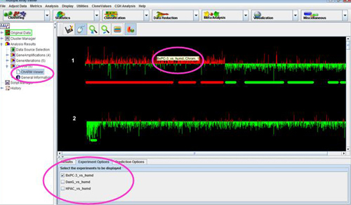
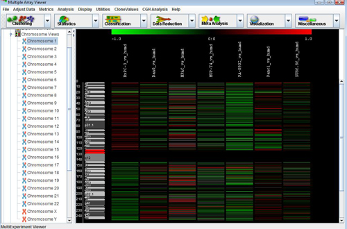
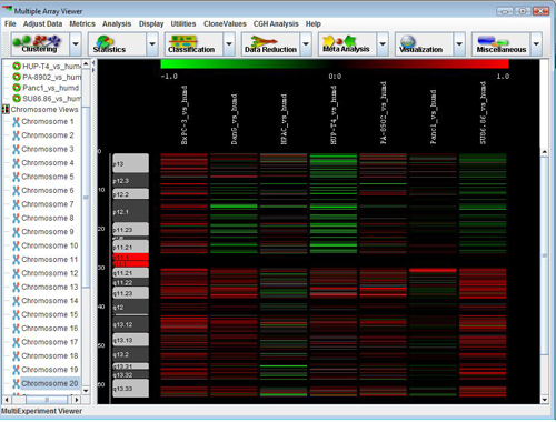
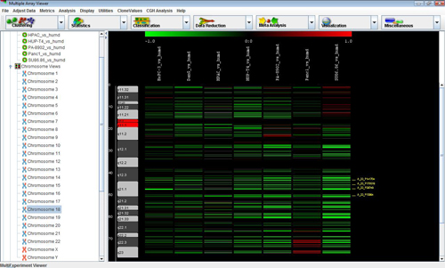
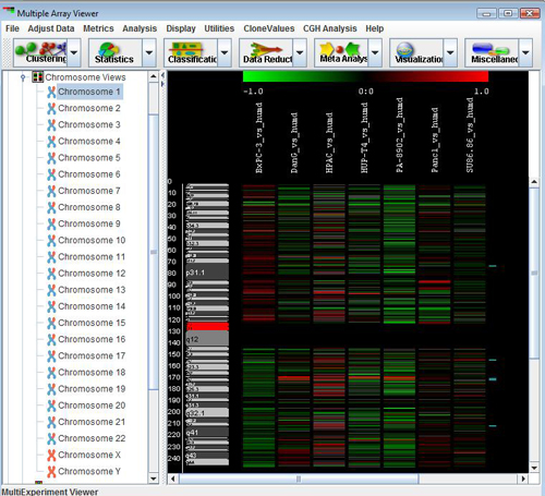
The node of the navigation tree should contain a subtree called . Expand this subtree to display a list of all chromosomes. Clicking on any of these chromosomes will display the CGH Position Graph Viewer for that chromosome.
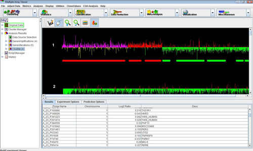
The CGH Position Graph Viewer is used to display data values for a single chromosome for multiple experiments. The left side of this view displays the cytogenetic bands of the selected chromosome. Positional coordinates, in MB, are annotated to the left of the cytobands. Probes are represented as horizontal bars beginning and ending at positions corresponding to the genomic coordinates of the clone.
Probes in this display are colored the same way as described for the Circle Viewer. Clone values, color schemes, and ratio scales can be adjusted.
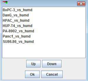
The order in which experiment appear in the display can be changed by using the item in the menu. The position of samples can be moved up and down using the buttons on the bottom of this dialog, and selecting will cause the experiments to be displayed using the new order.
The width and length of the probes can be changed through the and items in the menu. By default the width and length are calculated to fit the entire display on the screen. It is often useful to increase the length to look at a particular region because it is often difficult to distinguish probes that lie close to each other.
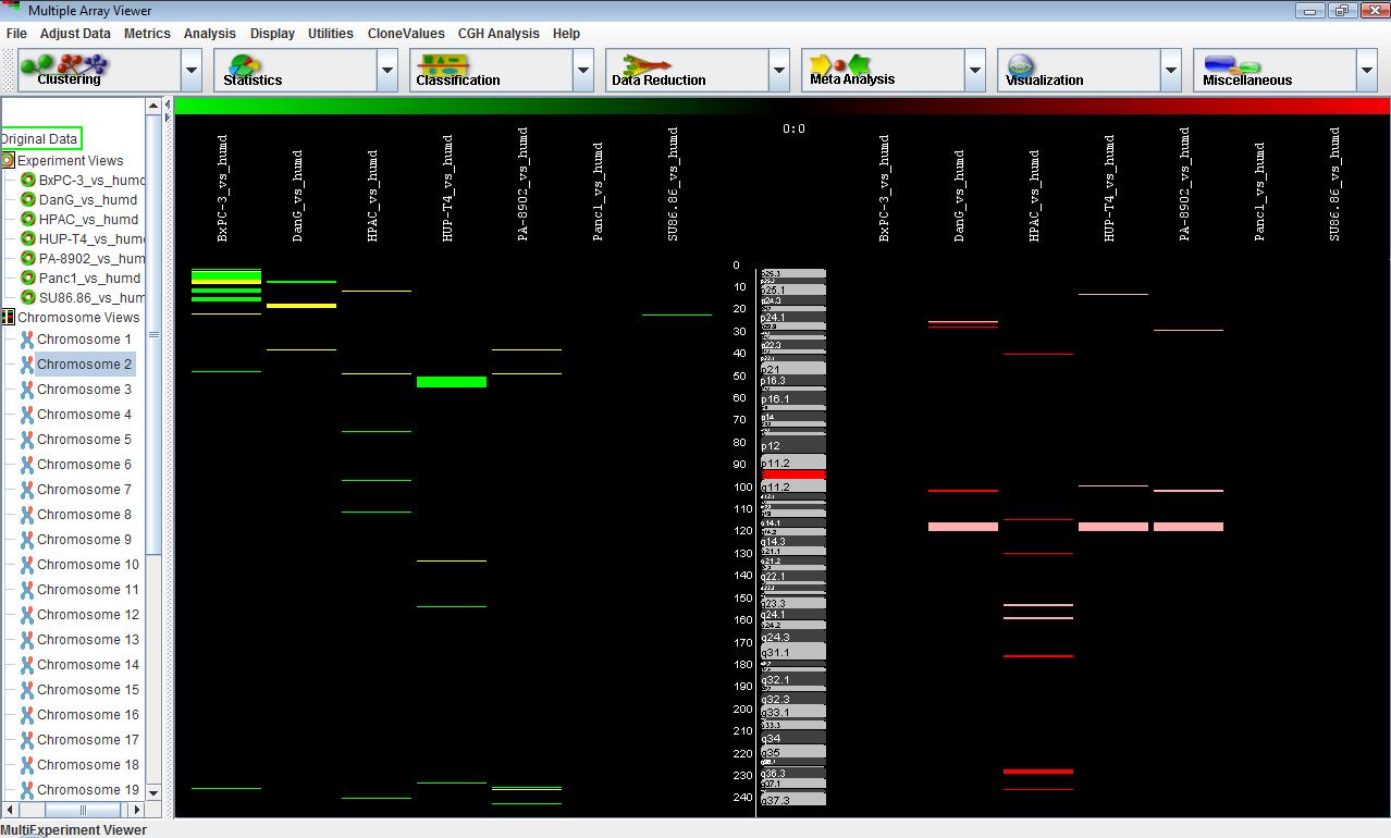
A common way to display CGH data is to draw all deletions on one side of the screen and all amplification on the other side. The separated view of the CGH Postion Graph displays the cytogenetic bands and chromosome positions in the center of the panel, the flanking regions corresponding to deletions on the left of the screen and the flanking regions corresponding to amplifications on the right side of the screen. To display this view, in the menu, select . This display often looks better if the element width item is set to a smaller value.
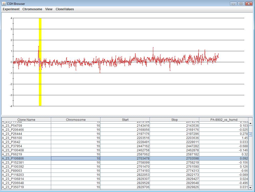
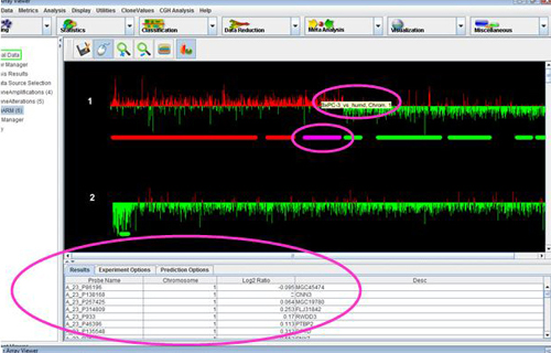
The CGH Browser displays a plot representation of one or more CGH experiments. Right clicking on any flanking region or probe in the CGH Position Graph Viewer, or on any probe in the CGH Circle Viewer and selecting will launch the CGH Browser with the values corresponding to the selected data region highlighted on both the chart and the table.
The menu of the CGH Browser can be used to toggle the display between each experiment that has been loaded, or all experiments. The menu of the CGH Browser can be used to toggle the display between one chromosome or all chromosomes.
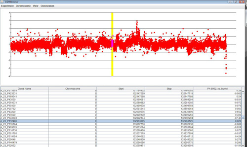
Clicking anywhere on the chart will highlight the data point closest to the selection, as well as the corresponding row in the table. Selecting any number of rows in the table will highlight the corresponding region in the chart. The View menu can be used to change annotations and display styles in the browser.
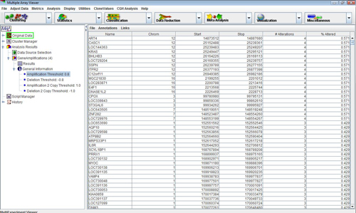
The CGH Analysis menu contains a number of algorithms for searching for data regions that are consistently altered throughout the experiments. These algorithms can be performed on probes, genes, and data regions (minimal common regions of alteration).
The items are used to search for probes that are commonly altered throughout the experiments. Click on the item. Notice that a subtree has been added to the Analysis node of the navigation tree on the left side of the screen. Expanding this tree and selecting the node will set the main view to display a table showing the number and percentage of experiments in which each clone is deleted.
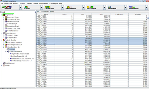
Highlight all of the probes on chromosome 1 with 4 or more alterations and select the item in the menu. This will set the selected data regions to be annotated in the corresponding CGH Position graph. Click on the item on the subtree of the navigation tree on the left side of the screen to see the selected probes annotated. The element length may have to be changed to view all annotated probes.
Right clicking on an annotation allows for querying of genes containing in the region, and to link to the CGH Browser with the selected annotation highlighted. If the CGH Browser corresponding to an annotation is displayed, it will display the log average inverted clone values for all experiments for the chromosome corresponding to the annotation.
Annotations can be cleared by using the item in the menu.
The Results of any CGH Analysis algorithm can be saved as a tab delimited text file. To do this select the Save item from the File menu of the algorithm results viewer.
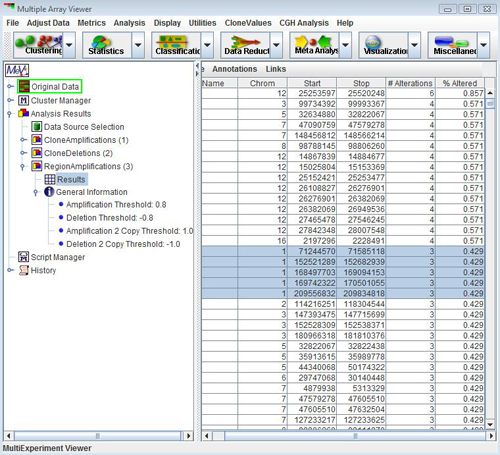
The items are used to search for common regions of amplifications and deletions. It is often important to identify minimal regions of alteration that are common between a number of experiments. Select the item.
Select and annotate these five regions, and display the CGH Position Graph viewer for chromosome 1. The annotated data regions are represented by light blue rectangles on the right side of the display. This technique can be used to significantly reduce the size of the data regions determined for further investigation. Right-click on any of the blue rectangles and select to check if there are any consistently deleted genes of interest. These are displayed in a tabular format.
The items and are used to search for genes that are commonly altered between experiments. Select the item. Select the node in the newly created subtree. This view displays the number of deletions for every gene stored in UCSC’s Golden Path database.
Selecting the item in the menu will calculate the number of amplifications and deletions for every gene in a customized gene list. Select this button and load the file named “CGH_sample_genelist.txt”, included with the distribution of the MeV. This list is a text file containing a large number of genes that have been identified as being associated with cancer. Notice that the new Gene Alterations subtree now contains two subtrees, corresponding to the number of times the genes in the list are amplified and deleted.
Nodes in any tree can be deleted. Right click on the node and select .
Selecting the item from the menu will display a dialog prompting for the name of a gene. Enter the name of a gene of interest and click . A dialog will appear showing how many times that gene is deleted and amplified in the dataset. Selecting from the menu of this dialog will display the CGH Position graph corresponding to this gene, with the gene annotated.
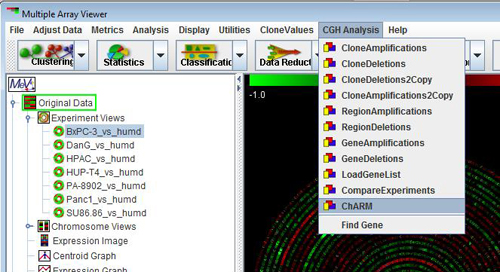
We have integrated a new module called ChARM, a robust expectation maximization based algorithm for identification of segments of chromosomal aberrations from CGH data. (ChARM, Meyers, C.L et al, 2004)
: Please follow the series of screenshots and any instructions associated with it to start the analysis.
1. After loading the CGH data navigate to the main menu “CGH Analysis” option and select “ChARM” from the drop-down.
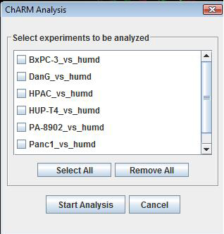
2. A new window opens which displays all CGH experiments that are loaded. Use the check boxes to select the experiments that needs to be analyzed and hit “Start Analysis”