BIRCH

return to tutorials

TUTORIAL: VISUALIZATION OF PHYLOGENETIC TREES


June  25, 2021


Archaeopteryx: $doc/forester/ArchaeopteryxUserDocumentation.pdf
Integrated Taxonomic Information System (ITIS)
 

This tutorial continues from the previous tutorial Phylogenetic Analysis Using Distance Methods. It begins with multiply aligned protein and DNA sequences for plant type III chitinases. To eliminate gappy positions, the alignments were processed by Gblocks. The starting point for this tutorial is the Gblocks output alignments.

Purpose: To demonstrate the power of tree visualization using Archaeopteryx. Archaeopteryx is very feature-rich, so we will only demonstrate some of its capabilities here.


1. The dataset

Create a new directory called trees. Save these files to the tree directory

Tree of Chitinase III DNA sequences - chitIII.CDS.pal2nal.gblocks.dnaml.phyloxml
Tree of Chitinase III protein sequences - chitIII.pro.mafft.gblocks.proml.phyloxml

We will go through the tutorial using the protein tree, and at the end compare the protein tree with the corresponding DNA tree.

2. Populating the tree with taxonomic metadata


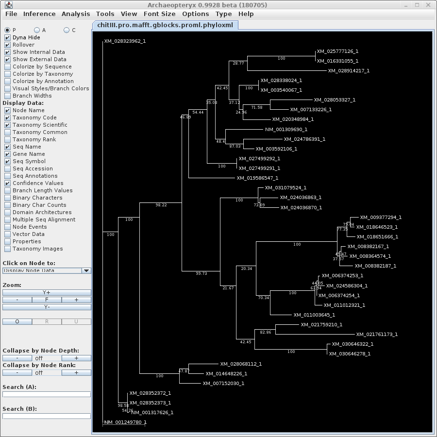
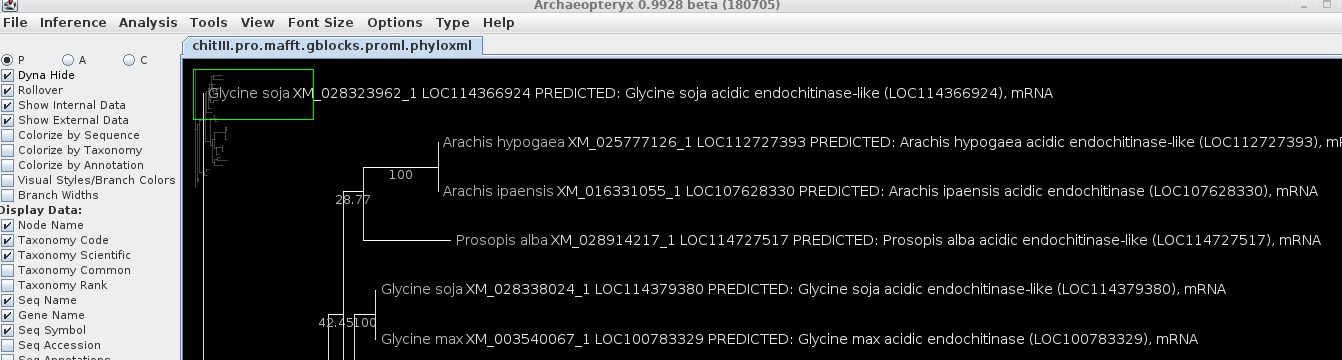
The phyloxml files contain only the Accession numbers of the sequences, the tree topologies, branch lengths, and bootstrap replicate numbers.

cd into the trees directory and launch blnalign. Launch Archaeopteryx either by typing 'archaeopteryx' at the command line, or from BIRCH --> Phylogeny.

In this case, we'd like to know the species from which each sequence is derived.

One of the great features of Archaeopteryx is the ability to retrieve this information from databases, using the accession numbers of the sequences in the tree.


This is done in two steps. First, choose Tools --> Obtain sequence information. You'll see a progress message


This sometimes takes several minutes. An OK box will pop up when retrieval is complete. Choose Font Size --> Large fonts to make the data readable.


These data come from the Description  and Source fields of the GenBank entries. For the purposes of assessing the evolution of these genes, we would like more complete taxonomic information on different taxonomic ranks (eg. genus, family order...). Choose Tools --> Obtain detailed taxonomic information.

These data do not appear, but will be used as we proceed.

This is a good point to save the tree, so that all this data will be retained in the phyloxml file. Choose File --> Save Tree As and give the file a new name so that we don't overwrite the original file. A short name should be fine: chitIII.pro.phyloxml.

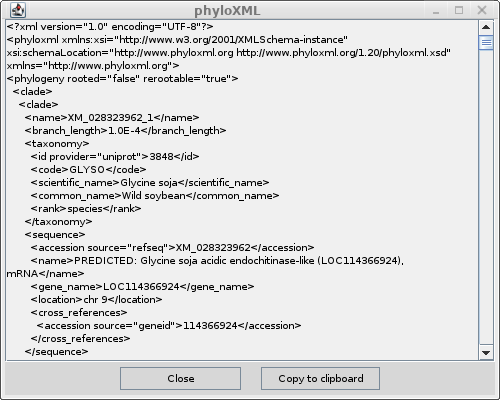
It is instructive to have a look at the XML code by choosing View --> as phyloxml.

If you have ever made web pages, you'll be familiar with XML. HTML is a subset of the more general XML format. For each type of data, there is an XML specification. So HTML is one kind of XML, phyloxml is an XML for specifying phylogenetic trees and associated metadata. The formal definition can be found at phyloxml.org.


3. Settings to help us learn more from our data

Typically, you don't need all of this data in the display, so let's turn off some of it. In the control panel at left uncheck the following boxes:  Taxonomy Code, Seq Name, Gene Name. Now only the genus/species name and the Accession number should remain.

The default font can be thin, and especially difficult to read in color, so change to boldface using Options --> Select default font, and then clidking on "Bold".

We can assign different colors to each species using Colorize by taxonomy on the control panel.

To get better visual contrast between labels and background, try different settings in Options --> Background color gradient and Options --> Select color scheme. This example uses the Orange color scheme.


Note the inset box at upper right. Move this box to view part of a large tree, or to re-center the tree to fit the window.

4. Comparison of protein and DNA trees

How different are the tree from the protein alignment and the tree from the DNA alignment? If you have a large enough screen, you can put the two Archaeopteryx windows side by side on your screen. A superficial glance at the two trees, especially when species are color-coded, makes them look very different.

However, a tree is a model that groups sequences based on similarity between pairs. A close examination of part of the tree illustrates that many parts of the protein and DNA trees are equivalent, even though the vertical order of sequences is different.

protein
DNA


For example, looking at the protein tree, we see a Vigna and Phaseolus sequence together on a terminal branch. The next deepest branch has two Glycine sequences together, and the next deepest branch has a sequence from Cajanus. If you examine the same clade on the DNA tree, you will see that the branching order (topology) is identical.

That means that it is perfectly legitimate to rotate any branch, which changes the vertical order of sequences on the tree, but not the tree topology. Put another way, swapping any branch does NOT change the branching order. It is still the same tree.

In other words, if we rotate (swap) branches on one or both trees, we can make the trees look more similar without changing branch length or topology.

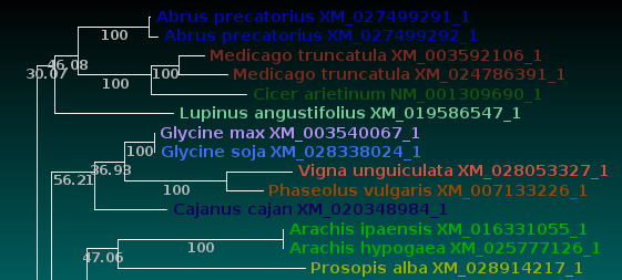
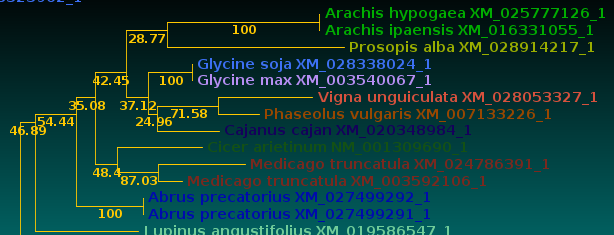
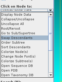
The Click on Node to: tool on the control 
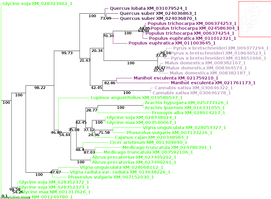
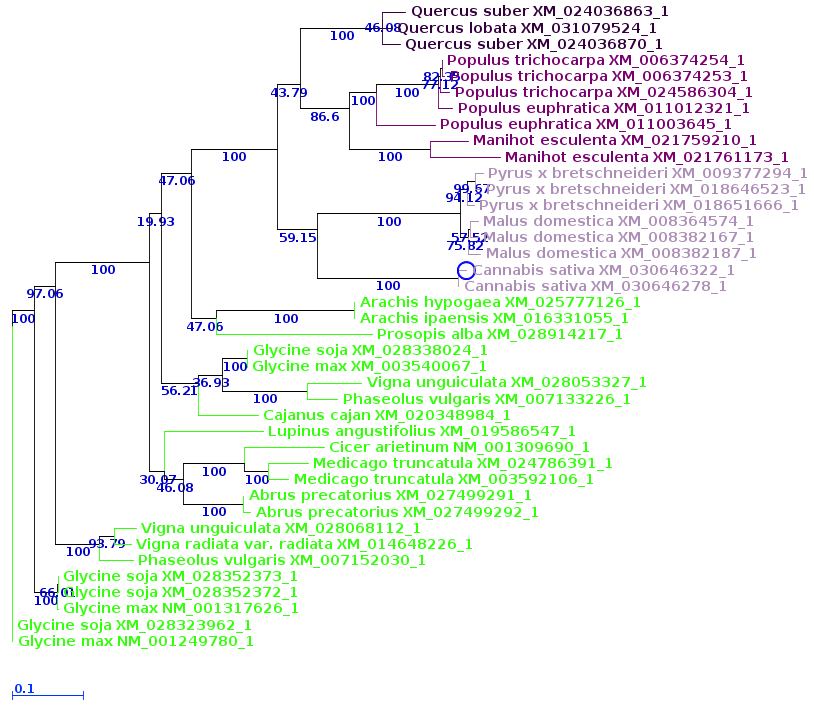
panel.

As a trivial example, the protein tree shows the Glycine soja sequence above the Glycine max, while the DNA tree show Glycine max above Glycine soja. To eliminate this meaningless difference between the two trees, click on the outer node joining the two Glycine sequences in the DNA tree:


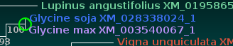
The green circle shows where the node was clicked to swap the branches.


With the protein and DNA trees side by side, click on internal nodes to swap groups of branches (clades), until the two trees look as similar as is possible to do. The best way is to begin at inner nodes and work your way out to the periphery of the trees.

protein
DNA


While the color scheme used was instructive for distinguishing species, some of the colors used don't show up well against the background. To make for better readability, turn off Options --> Color gradient and change Options --> Select color scheme to "Simple".

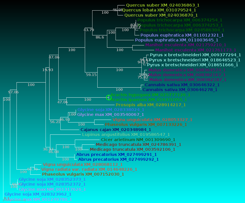
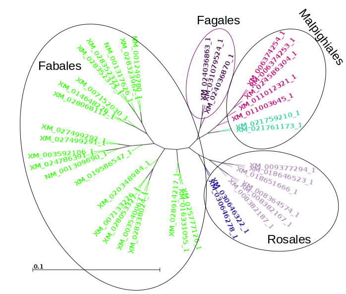
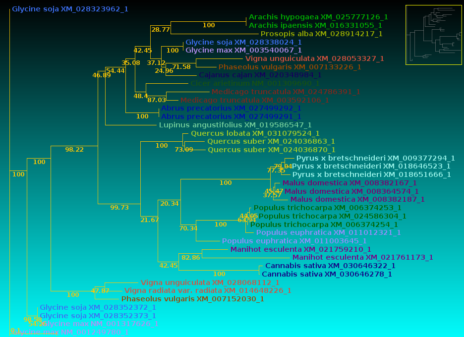
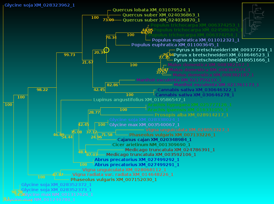
Now, let's compare how the protein and DNA trees separate species based on a higher taxonomic rank.
 
For both protein and DNA trees, Tools --> Colorize subtrees by taxonomic rank, and choose "Family".

The most striking thing shown in the comparison is that while the protein alignment groups the sequences from Manihot (Cassava, order Malpighiales) with Pyrus, Malus and Cannabis (order Rosales), the DNA tree groups Manihot with Populus, which is also in Malpighiales. Bootstrap values indicate that Populus and Manihot were together on 86.6% of replicate trees.
order family genus
Fagales Fagaceae Quercus
Malpighiales Salicaceae Populus
Malpighiales Euphorbiaceae Manihot
Rosales Rosaceae Pyrus
Rosales Rosaceae Malus
Rosales Cannabaceae Cannabis
Fabales Fabaceae Arachis
Fabales Fabaceae Prosopis
Fabales Fabaceae Glycine
Fabales Fabaceae Phaseolus
Fabales Fabaceae Vigna
Fabales Fabaceae Cajanus
Fabales Fabaceae Lupinus
Fabales Fabaceae Cicer
Fabales Fabaceae Medicago
Fabales Fabaceae Abrus

protein
DNA


5. Generating figures for publication

What looks good on a computer screen often doesn't work for publication. In particular, the color-on black trees that make things stand out on the screen don't work well in a publication.

A few guidelines for publication:
At the end of the day, no program will do everything you want to do to get across the point you want to make with your figure. It will almost always be necessary to import your tree image into a drawing program to add things like labels, arrows, circles or brackets.

The example below was done as follows:  Choose Type -->  "Unrooted" and Options --> Radial labels. Also, uncheck Taxonomy Scientific on the control panel. This will leave only the Accession numbers on the tree, but will fit better in the space available.

Although Archaeopteryx has an option to export trees as bitmap graphics, the problem is that the tree often appears as a small area on a large "sheet of paper". A better solution is to take a snapshot of the Archaeopteryx windown itself and then crop out everything other than the tree, and save to a bitmap file such as PNG or JPG.

This file can then be imported into any drawing program to add annotation. The example below was done using GIMP on Linux to capture and crop the image, which was then imported into LibreOffice Draw for final processing.


In practice, it might also be necessary to turn off colors for the tree, which might not reproduce as well as black and white.

In conclusion, start with the idea you want to get across, and plan your tree to bring out that idea.