Assignment 1 (Sept.
26, 2024)
Comparative Genomics
This assignment is worth 20% of the course grade.
Due: Tuesday October 8, 2024.
Background 1,2
DNA replication in circular prokaryotic
genomes begins at a single origin of replication,
often visualized as being at 12 o'clock on the circle. Two
replication forks propagate in opposite directions,
and replication continues until they meet at the terminus,
visualized as being at 6 o'clock on the circle.
In bidirectional replication, each replication fork has both
a leading and lagging strand. As the two strands f and c are
"peeled apart", DNA synthesis on the leading strand proceeds
uninterrupted, while on the lagging strand, DNA must be
replicated in short stretches, referred to as Okazaki
fragments, which are initiated as the DNA duplex opens up.
|
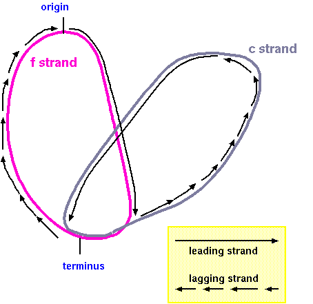
Figure1
|
Thus, as shown in Figure 2, we can define two
regions of a circular chromosome, arbitrarily designated A
and B, as illustrated at right. If the total length of the
bacterial chromosome was L, then region A would span
coordinates 1 to L/2, and region B would span coordinates
(L/2+1) to L.
Referring to Figure 1, in region A the f strand is template
for leading strand synthesis, and in region B, the c strand
is the template for leading strand synthesis.
|
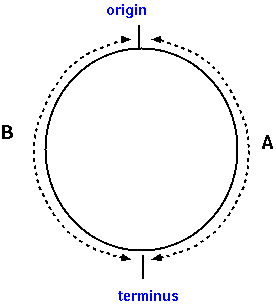
Figure 2 |
It has been observed that the leading strand tends to be enriched
for G, relative to C, particularly at the 3rd positions of codons.
There are several proposed mechanisms to explain this observation,
all resulting from the extra time that the lagging strand remains
single-stranded during DNA replication, relative to the leading
strand.1,2. The resultant G-C skew is therefore a
good indicator of which strands are the leading and lagging strands
in genomic DNA.
Genome viewers such as Artemis are powerful tools for understanding
genome organization and evolution. Artemis is designed to
superimpose different types of sequence features and graphs onto the
genomic map. In these displays, the relationships between sequence
characteristics and features become apparent. In this assignment, we
will use Artemis to explore the relationship between GC-skew, genome
organization, and transcription.
1. Create a symbolic link to the
genomes directory and a list of files to use
The directory /home/plants/frist/courses/bioinformatics/as1/genomes
contains a number of GenBank files, each for a different prokaryotic
genome. If you were to copy these files to your own directory, you
would probably exceed your disk quota. Instead, make a symbolic link
to the genomes directory, so that you can easily read these files.
cd $HOME/public_html/PLNT4610/as1
ln -s
/home/plants/frist/courses/bioinformatics/as1/genomes |
go to your as1 directory
create a symbolic link
|
The genomes directory will behave, for most purposes, as if it was
actually present in your as1 directory. For example, if you run
artemis in your as1 directory, when you open a file, the genomes
directory will appear to be present.
There are two ways in which the symbolic link will behave
differently. If you type 'ls -l genomes', you would see the link
itself, not the contents of the directory. To see the contents you
would have to include the -L option in the ls command ie. 'ls -lL
genomes'. The other point is that the genomes directory and
its contents are not world-writable. That means you can't create
files within that directory, nor can you delete or modify files in
that directory.
Each student will use 10 of the sequences in the genomes directory
for use in steps 2 - 4 of this assignment. So that each student may
have a unique set of sequences, download randomlists.sh
and save it in your as1 directory. Make sure that it is executable:
chmod u+rx randomlists.sh.
Next run the script (./randomlists.sh),
which will write your list to a file called AS1seqs_1.nam.
These are the sequences you will work with.
2. (4 points) Create a DNAPlotter Map
and save feature information for each sequence
a. DNAPlotter Map
For each genome in your list create a DNAPlotter Map. Make sure to
include a track for each of the following:
- coordinates and tick marks
- CDS (coding sequence) features on the forward strand
- CDS (coding sequence) features on the reverse strand
- tRNA, forward strand
- tRNA, reverse strand
- rRNA, forward strand
- rRNA, reverse strand
- rep_origin (origin of replication)
- GC plot
- GC skew plot
Feel free to use some creativity with colours and other settings
that make it easy to visualize features in the map.
Save your maps as PNG files for inclusion in your report. In
DNAPlotter, choose File --> Save as jpeg/png Image. Use
the ".png" extension to distinguish the plot file from the GenBank
file. For example, if the Genbank file was
Corynebacterium_ulcerans0102.gen, then your map should be saved as
Corynebacterium_ulcerans0102.png.
After producing your first map, export your tracks, as described in
the DNAPlotter
tutorial, to a file whose name includes ".tracks" as an
extension. You can import this file to speed up production of your
other genome maps.
b. Feature Information
For each genome, save the feature information by going to the
feature window in Artemis, right clicking on the mouse, and choosing
Save List to File. Use the ".fea" extension to distinguish
the plot file from the GenBank file. For example, if the Genbank
file was Corynebacterium_ulcerans0102.gen, then your map should be
saved as Corynebacterium_ulcerans0102.fea.
3. (5 points) Modify the existing
fea2tsv.sh script to read a feature list from Artemis, and
convert it into a Tab-Separated Value (TSV) file.
We can automate procedures using Unix commands by writing those
commands in a file referred to as a script. A script implementing
steps 1 -5 from the tutorial Extracting
features from text files can be found in the file fea2tsv.sh. In this exercise, we'll modify
the script with some improvements on the original protocol.
The problem is as follows: In the Background section above, we
have oversimplified things by assuming that for all prokaryotic
genomes, the replication origin will always be annotated as
starting at position 1. However, the choice of which nucleotide in
a circular genome gets specified as position 1 is often an
arbitrary location for many genome projects. Consequently, many
prokaryotic genomes place the replication at a different position.
For this reason, it would be far easier to calculate the f and c
values if our TSV file contains annotation for both CDS and
rep_origin features.
Fortunately, the grep command can read a file containing a list
of patterns, each on a separate line. The output from grep will be
any lines from that match any of the patterns. For example, you
could create a pattern file called fealist.txt containing the
following lines:
If we typed
grep -f fealist.txt < Corynebacterium_ulcerans0102.fea
any lines beginning with either CDS or rep_origin would be
printed to the standard output. (In regular expressions, '^'
indicates the beginning of a line. If '^' was not included in the
expression, the search would match any line that included CDS or
rep_origin anywhere within a line.)
To get started, save this file in your as1 directory. You
will need to make this file executable in order to run the script:
chmod u+x fea2tsv.sh
Before changing anything, try running the unmodified script yourself
using one of the feature files generated using Artemis. For example,
if your feature file is Corynebacterium_ulcerans0102.fea, you can
run the script by typing
| ./fea2tsv.sh Corynebacterium_ulcerans0102.fea |
By
default, the current working directory is not in your
$PATH. Therefore, when we run a script in the current
directory, we have to precede its name with ./
to tell the shell that the script is in the current
directory.
|
In this example, output would be written to a file called
Corynebacterium_ulcerans0102.fea.tsv.
Your job is to modify the script as follows:
- change the grep command in the script to read patterns from a
file specified in the grep command
- add a second command line argument that lets you type the name
of the pattern file as the second command line argument. You
will have to modify your grep command to read the specified
file. That makes the script more versatile, because you could
re-run it any number of times with different pattern files, to
get different tsv files.
The script is heavily annotated with comment lines ie. lines
beginning with a hash mark (#), that explain what each section of
code is doing. Places where you need to make changes have comments
in ALL CAPS to tell you what changes need to be made.
When the script is complete, you should be able to run it as in the
example below:
command
|
output file name
|
./fea2tsv.sh
Corynebacterium_ulcerans0102.fea fealist.txt
|
Corynebacterium_ulcerans0102.fea.tsv |
If you implement both modifications above, your script should be
able to read ANY file containing feature lines, not just
fealist.txt.
Your TSV file should directly readable by LibreOffice Calc without
any modification. Links to some useful tutorials for writing bash
shell scripts can be found in the References 3,4,5
below.
Before proceeding to the next, step, use your fea2tsv.sh script to
generate a .tsv file from each of your .fea files.
4. (5 points) Quantify transcriptional
strand biases for coding sequences.
For each genome, the goal is to quantify the transcriptional
bias, that is, the tendency for coding sequences to be transcribed
on either the forward or reverse strands, for each of the two
regions, A and B, as illustrated in Figure 2 above.
a. Decide on a cut off row that
delineates the junction between regions A and B
You can find the length of the genome on the LOCUS line of the
GenBank file for each genome. This information is also found in
Artemis, using View --> Overview. The replication
terminus can be assumed to be at the half way point on the circle,
opposite the replication origin. That is, if the origin is
position 1, and the sequence is length L, then the terminus would
be at position L/2. For example, if the sequence was 2,500,000
bases long, the terminus would be at position 1,250,000.
If the
replication origin (R) was at a position other than 1, you
would have to calculate the terminus based on that position.
|
Calculate the halfway point H = floor(L/2)*.
The location of the terminus T is given as follows:
if R > H
:
T = R - H
else:
T = R + H
|
*The
floor function rounds a real number down to the nearest
integer. In the case of R = H, we would get a T value
greater than the length of the sequence if L/2 was rounded
up.
|
Next, scroll down the rows of your spreadsheet to roughly the
halfway point. Look for a coding sequence whose coordinates
overlap the terminus. This row would be the last row in region A.
The next row would be the starting point for region B. For
example, if there were 4000 CDS sequences total, region A might
span rows 1 through 1987 in the spreadsheet, and region B would
span rows 1988 through 4000.
What if no rep_origin
feature is present?
Not all species have an annotated rep_origin feature. In
these cases, you can make a rough guess as to the location
of the origin based on the GC skew plot. Use that as your
presumptive origin of replication.
|
b. Calculate the transcriptional bias
for regions A and B.
The transcriptional strand bias (TSB) is the degree to which the
direction of transcription is skewed either to the forward strand
or the reverse strand. It could be calculated as a ratio of the
difference between numbers of CDS features on the forward and
reverse strands to the total number of coding sequences in each
region. That is,
TSB = (f-c)/(f+c)
where
- f is the number of CDS features on the forward strand
- c is the number of CDS features on the complementary strand
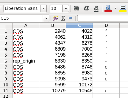
Suppose you had the following data in your spreadsheet:
If the CDS sequences in region A spanned the first 5 rows, and
those in region B spanned the last 5 rows, you could calculate the
TSB values for each region.
For example, to calculate TSB for region A in LibreOffice Calc,
you could count the number of CDS features on the forward strand
using the formula =COUNTIF(D1:D5,"f"). Similarly the number of CDS
features on the complementary strand would be counted using
=COUNTIF(D1:D5,"c"). Region B would be calculated similarly.
In your report, the results would be shown in a table for each
species.
region
|
|
|
(f-c)/(f+c) |
A
|
f(1:5) = 5
|
c(1:5) = 0
|
1.0
|
B
|
f(7:10) = 1
|
c(7:10) = 4
|
-0.6
|
Save your spreadsheet in LibreOffice Calc format, by choosing
File --> Save As. In the Save window, choose "ODF Spreadsheet
(.ods) as the format, and Save. For example, if the file you read
into the spreadsheet was Corynebacterium_ulcerans0102.fea.CDS.tsv,
the file would be exported to
Corynebacterium_ulcerans0102.fea.CDS.ods.
5. (3 points) Conclusions - What have you
learned?
- Are there any generalizations you can make about GC skew among
these species? What are the exceptions?
- What do the observations about GC skew and transcriptional
strand bias tell us?
- What distinguishes the Candidatus Hamiltonella defensa genome
from the other genomes?
- Although prokaryotic genomes are circular, linear genomes have
been observed in some species. Check the LOCUS lines of your
GenBank files to see if any of the genomes in your sample are
linear. If one of your genomes is linear, is there anything
unique about the results for that genome, or the results
generally similar to those for circular genomes?
6. (3 points) Presentation.
Part of the grade will be determined by the quality of your
web page(s) for the assignment, including:
- The assignment page(s) must be accessible at
http://home.cc.umanitoba.ca/~userid/PLNT4610/as1/as1.html.
No other URL will be accepted.
- All links must work, and all graphics must display. Each time
I have to contact you to fix something, 1 point will be
deducted. You get no credit for anything I can't access.
- Pay attention to the organizational and stylistic hints found
in Lecture
2. Do what it takes to make it easy to read and to
understand the points you wish to get across.
How to get
started
1. Create a directory called either
public_html/PLNT4610/as1 or public_html/PLNT7690/as1. Make this
directory world-readable and world executable. (That's as1 - using
the number 1, rather than the letter l).
2. Do all work in the as1
directory. That way, all your files will already be where they
need to be.
What
you need to complete your assignment
Your report should include the following:
1. Links to your tracks file and your fea2tsv.sh script, and a
link to your AS1seqs_1.nam file.
2. For each genome, present your results in a 2-column table,
as shown in the sample file.
You are expected to follow the file naming conventions used
above. To make it easier to compare results between species, put
all maps and TSB calculations on a single page. Do not make
separate pages for each species.
3. A discussion of the main findings from your data. The questions
in part 5 above are a starting point, but feel free to add
additional observations, explanations, or to state hypotheses
arising from the observations. Feel free to make tables, charts,
graphs, or anything that will get your points across.
How to post it (3 points)
1. Create a new HTML file called as1/as1.html. Your web page
for Assignment 1 should take the form of a report, that makes it
easy to figure out what you did.
2. Make all files in the as1 directory world-readable. (chmod
a+r *)
3. Edit either PLNT4610.html or PLNT7690.html to include a link
to as1/as1.html.
4. In the Firefox or SeqMonkey Browser, go to your home page
and follow all hypertext links to your assignment, and test all
links to your output files.
On the day the assignments are due, I should be able to just go
to each person's web site and find the output. You don't need to
send me an email message saying that your assignment is complete.
If you choose not to hand in this assignment, you don't need to do
anything.
Academic integrity:
1.Your work is assumed to be your own original work. All
University policies regarding academic integrity apply.
2. Show your work. For example, a spreadsheet that had the
final answer typed in, rather than calculated by a formula, would
not provide any evidence that you had actually done the work.
References
1. Francino MP, Ochman H (1997) Strand asymmetries in DNA
evolution. Trends in Genetics 13:240-245.
2. Mclean MJ, Wolfe KH, Devine KM (1998) Base Composition Skews,
Replication Orientation, and Gene Orientation in 12 Prokaryotic
Genomes. J. Mol. Evol. 47:691-696.
3. BASH Programming - Introduction HOW-TO [http://tldp.org/HOWTO/Bash-Prog-Intro-HOWTO.html]
4. Chadwick, R (2015) Bash Scripting Tutorial - Ryan's
Tutorials [http://ryanstutorials.net/bash-scripting-tutorial/]
5. Gite, V. (2015) Learning bash scripting for
beginners [http://www.cyberciti.biz/open-source/learning-bash-scripting-for-beginners/]