Lecture 7, part 3 of 4
| PLNT4610/PLNT7690
Bioinformatics Lecture 7, part 3 of 4 |
Consider a set of 5 DNA
sequences:
| Algorithm: build a starting tree by connecting any two sequences to form a branch while (not all sequences are added) choose the next sequence add this sequence to the tree swap branches to find tree with fewest mutations re-calculate branch lengths |
As each sequence is
added, we swap branches and find the optimal tree for the
current group of sequences. Doing the optimization in the early
steps when the tree is small, greatly reduces the size of the
task when later branches are added. That is, we eliminate from
future steps the large number of branchings to consider that
could not possibly lead to trees that are more parsimonious than
the current tree.
The output from the PHYLIP DNAPARS program [testphyl.dnapars.outfile ] lists 3 most parsimonious trees, each requiring a total of 13 substitutions to traverse the entire tree. One such tree is:
                         +-Epsilon
  +----------------------2
  |                      +------Delta
  |
  1-------------Gamma
  |
  +-Beta
  |
  +-----------Alpha

requires a total of     13.000

  between      and       length
  -------      ---       ------
     1           2       0.384615
     2      Epsilon      0.038462
     2      Delta        0.115385
     1      Gamma        0.230769
     1      Beta         0.038462
     1      Alpha        0.192308

steps in each site:
         0   1   2   3   4   5   6   7   8   9
     *-----------------------------------------
    0|       2   0   1   2   0   2   1   0   0
   10|   1   0   1   3
Name            Sequences
----            ---------

Alpha        AACGTGGCCA CAT
Beta         ..G..C.... ..C
Gamma        C.GT.C.... ..A
Delta        G.GA.TT..G .C.
Epsilon      G.GA.CT..G .CC
The point of maximum parsimony is that, although sequences could be placed at any position on the tree, the number of steps required to interconvert one sequence to another changes each time branches are moved. Thus, the most parsimonious tree is the tree whose topology requires the fewest total mutations.
Advantages
Disadvantages
- reconstructs ancestral nodes, thereby using all the evolutionary data
- has been shown to perform better than distance methods using simulated data and real data from pedigrees
- provides numerous "most parsimonious trees"
- branch lengths can not be reliably determined, only topology (actually, no longer true. See Hochbaum and Pathria (1997) Path costs in evolutionary tree reconstruction. Journal of Computational Biology 4:163-175. This method used in PHYLIP programs DNAPARS and PROTPARS)
- slower than distance methods
- provides numerous "most parsimonious trees"
- sensitive to order in which sequences are added to tree
3. Maximum Likelihood (ML)
The term Maximum Likelihood does not refer to a single statistical method, but rather to a general strategy. Most analytical methods begin with data and work towards an answer. ML methods take what has been described as an "inside out" approach. In their simplest form, they begin by listing all possible models, and then calculating the probability that each model would generate the data actually observed. The model with the highest probability of generating the observed data is chosen as the best model.
The algorithm could be stated something like this:
PB = P(alignment | T[1])
for each possible tree T[n]
PM = P(alignment | T[n])
if PM > PB
PB = PM
arbitrarily choose a tree and calculate the likelihood that that tree would result in the observed alignment
repeat for every possible tree:
choose a new tree and calculate the probability
PB is the probability of the best tree so far
Joe Felsenstein's application of ML to phylogeny is implemented in DNAML in the PHYLIP package. DNAML works by successive addition of sequences to a tree, optimizing the tree by maximum likelihood at each step. Each site (column) in the alignment is considered separately as illustrated in the figure below:
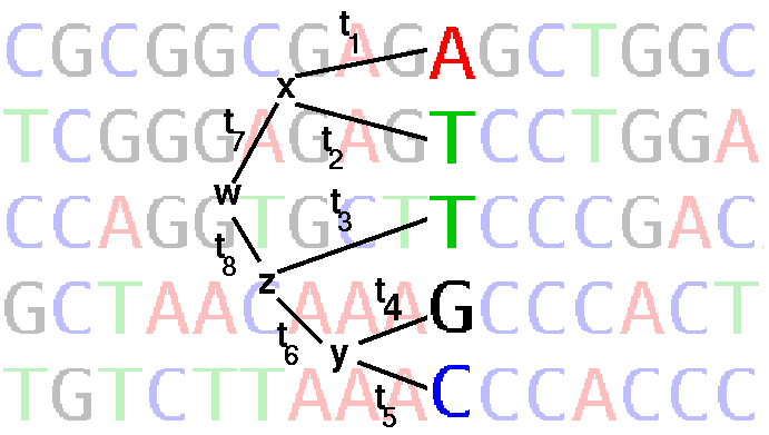
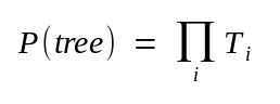
where ti are branch lengths (ie. rate of base substitution times time)
Ti ::= The probability that this position in the alignment contains exactly the nucleotides ATTGC is the sum of the probabilities of all possible ways of getting to those nucleotides via different hypothetical ancestors, whose (unknown) nucleotides are x, y, z, and w. This assumes independence of lineages and sites (Paraphrased from J. Felsenstein)
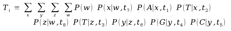
where terms like P(z | w,t8) refer to the probability of observing the nucleotide at node z, given the nucleotide at node w and branch length t8. These terms depend on the probability model of base change over time.
The probability of the tree is then given as
Calculate the probability of seeing exactly this tree by multiplying Ti values from each position in the alignment, given the tree.
from J. Felsenstein [http://www.cs.washington.edu/education/courses/590bi/98wi/ppt16/sld015.htm ].
The individual probabilities of a given mutation, going from one node to another, are based on observed base frequencies. Thus, the likelihood of seeing precisely these nucleotides at the terminal branches is the sum of the probabilities of substitutions at each node in the tree, at that one position. Finally, the probabilities for all sites are multiplied together to give the probability of the entire alignment, given that tree.
DNAML output using the same five sequences Alpha - Epsilon as in the previous example, is shown:
Nucleic acid sequence Maximum Likelihood method, version 4.0


Empirical Base Frequencies:

   A       0.24615
   C       0.36923
   G       0.21538
  T(U)     0.16923

Transition/transversion ratio =   2.000000


                                       +Epsilon
  +------------------------------------3
  !                                    +---------Delta
  !
  !  +Beta
--2--1
  !  +-------------------Gamma
  !
  +-----------------Alpha


remember: this is an unrooted tree!

Ln Likelihood =   -60.05644

 Between        And            Length      Approx. Confidence Limits
 -------        ---            ------      ------- ---------- ------

   2          Alpha             0.30389     (     zero,     0.68289) **
   2             3              0.61975     (     zero,     1.28978) **
   3          Epsilon           0.00006     (     zero,     0.26048)
   3          Delta             0.16586     (     zero,     0.40674) **
   2             1              0.00006     (     zero,    infinity)
   1          Beta              0.00006     (     zero,    infinity)
   1          Gamma             0.33972     (     zero,     0.77181) **

     *  = significantly positive, P < 0.05
     ** = significantly positive, P < 0.01
Advantages
Disadvantages
- reconstructs ancestral nodes, thereby using all the evolutionary data
- generates branch lengths
- generates statistical estimate of significance of each branch
- has been shown to perform better than distance methods using simulated data and real data from pedigrees
- VERY slow! Time required increases roughly with the fourth power of the number of sequences. Only practical with small numbers of sequences.
D. Evaluating Phylogenies
It is important to remember that the output from phylogenetic analysis is one answer obtained using one set of conditions. Even when an alignment has been carefully crafted and conditions such as substitution matrices or scoring methods are carefully chosen, it is possible to generate a meaningless tree. All other reasons aside, the input data may simply not be robust. That is, the data itself may contain more noise than evolutionary signal. We describe here two ways to test phylogenies.1. Jumbling sequence addition order
Most methods for phylogeny construction are sensitive to the order in which sequences are added to the tree. Consequently, the simplest way to test a phylogeny is to repeat the analysis several times with different addition orders. All PHYLIP programs, and most other phylogeny programs, have an option called JUMBLE, that uses a random number generator to choose which sequence to add at each step, rather than adding them in the order in which they appear in the file. The user is asked to supply a random number to use as a "seed" in generating a random number chain.It is especially important to remember that the order in which sequences appear in a file is often not random. For example, a sequence file used in an alignment might contain sequences from each species grouped together in the file. Non-random sequence order might therefore introduce a bias into the dataset. Therefore, even when doing only one run on a phylogeny, it is probably a good idea to jumble the order of sequences.
2. Bootstrap and Jacknife replicates
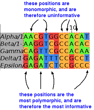
One of the fundamental problems with phylogenetic inference is that we are stuck with a single set of data, of finite length. We have no way of knowing whether the tree inferred from the data is truely representative of the evolutionary history of the gene family. To make matters worse, not all positions in an alignment are informative. That is, some positions are invariant, and therefore make no contribution to the phylogenetic tree. In particular, when sequences are short or polymorphism is minimal, we can have little confidence that the tree inferred from that data is the correct one.
Ideally, we would like to have a very long alignment with many polymorphic sites, so that no one site, or small number of sites in the alignment, would be heavily weighted in constructing the tree. Put another way, the more data, the less likely it is for an artifactual phylogeny to be produced.
In the example at right, perfectly conserved positions ie. monomorphic, are the same in all sequences, which suggests that no mutational events have occurred at these positions.
Other positions show evidence of at least 3 mutational events, and are said to be highly polymorphic.
These positions are highly informative, because they contain a lot of evolutionary information.
The remaining positions (eg. 3) display fewer mutational events, and are less informative.
In summary, the more mutational events seen at a site, the more information that is available for reconstructing a phylogeny.
The statistical method of bootstrapping is based on the assumption that the statistical properties of a sample should be similar to the statistical properties of the population from which that sample was drawn. The larger the sample, the more representative it should be of the population. Conversely, if the original sample was large enough, it should also be possible to take smaller samples from the larger sample, and expect that the smaller samples would also retain most of the statistical properties of the original population.
This is the assumption upon which the method of Jacknife resampling is based. If you repeatedly took random samples of the dataset, the resultant small data subsets should give you the same answer as the original large dataset. In the case of phylogenies, if we create smaller alignments containing only some of the positions from the total alignment, and use these mini-alignments to construct a tree, we should still get the same tree each time. This gives us a way of assessing how strongly a tree is supported by the data. If we get the same tree each time the data is sampled, then we are strongly confident that all the data is consistent with the tree. If we get a different tree with each sample, then no tree is strongly supported by the data.
Jacknife resampling has the drawback that the subreplicates are of a smaller size than the original dataset, which may change the statistical properties of the samples. For that reason, Jacknife resampling has largely been replaced by bootstrap resampling.
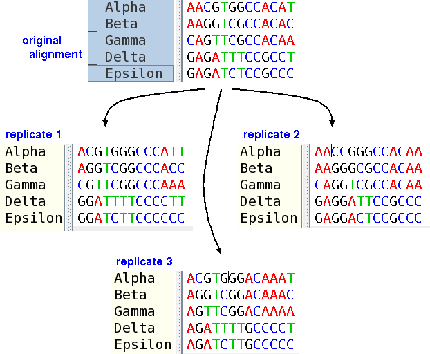
Bootstrap resampling is sampling with replacement. In the case of a multiple sequence alignment, sites are sampled at random until the dataset is equal in length to the original alignment.
To illustrate bootstrap resampling, in replicate 1, positions 2 (AAAAA), 10 (AAAGG) and 11 (CCCCC) have been deleted, while positions 7 (GGGTT), 9 (CCCCC) and 13 (TCATC) have been duplicated.
To give another example, a short DNA sequence alignment is shown below. Red asterisks signify the number of times a position is represented in the dataset. In the original dataset, each site is represented once.
ORIGINAL DATASETTwo examples of bootstrapped datasets, based on this alignment are shown below.
**************************************************
10 20 30 40 50
consensus AtngccatctAttGGGGcCAAaAcGgnaacGAaGGnncnctngcngacaC
CACHIT attgcagtgtattggggacaaaatggaaatgaagggtctttgcaagatgc
PSTCHIT atagctgtttactggggccaaaacggtggagaaggatccttagcagacac
NTACIDCL3 atagtaatatattggggccaaaatgggaatgaaggtagcttagctgacac
S66038 attgtcatatactggggccaaaatggtgatgaaggaagtcttgctgacac
CUSSEQ_1 atcgccatctattggggccaaaacggcaacgaaggctctcttgcatccac
CUSSEQ_2 atcgccatctattggggtcaaaacggcaacgagggctctcttgcatccac
CUSSEQ_3 atcggcatctattggggccaaaacggcaacgaaggctctcttgcatccac
VIRECT atttccgtctactggggtcaaaacggtaacgagggctccctggccgacgc
VURNACH3A auuuccgucuacuggggucaaaacggcaacgagggcucucuggccgacgc
ATHCHIA atagccatctattggggccaaaacggaaacgaaggtaacctctctgccac
VURNACH3B auagccaucuacuggggccaaaacggcaacgagggaacgcuuuccgaagc
NTBASICL3 attgtagtctattggggccaagatgtaggagaaggtaaattgattgacac
BOOTSTRAP REPLICATE 1* *
* * * * * * * *
*** ********* ** * *** *** * **** ***** **** ****
10 20 30 40 50
consensus AtngccatctAttGGGGcCAAaAcGgnaacGAaGGnncnctngcngacaC
CACHIT attgcagtgtattggggacaaaatggaaatgaagggtctttgcaagatgc
PSTCHIT atagctgtttactggggccaaaacggtggagaaggatccttagcagacac
NTACIDCL3 atagtaatatattggggccaaaatgggaatgaaggtagcttagctgacac
S66038 attgtcatatactggggccaaaatggtgatgaaggaagtcttgctgacac
CUSSEQ_1 atcgccatctattggggccaaaacggcaacgaaggctctcttgcatccac
CUSSEQ_2 atcgccatctattggggtcaaaacggcaacgagggctctcttgcatccac
CUSSEQ_3 atcggcatctattggggccaaaacggcaacgaaggctctcttgcatccac
VIRECT atttccgtctactggggtcaaaacggtaacgagggctccctggccgacgc
VURNACH3A auuuccgucuacuggggucaaaacggcaacgagggcucucuggccgacgc
ATHCHIA atagccatctattggggccaaaacggaaacgaaggtaacctctctgccac
VURNACH3B auagccaucuacuggggccaaaacggcaacgagggaacgcuuuccgaagc
NTBASICL3 attgtagtctattggggccaagatgtaggagaaggtaaattgattgacacBOOTSTRAP REPLICATE 2* *
* * * * * * *
********* ***** **** * ******** * *** *** * ******
10 20 30 40 50
consensus AtngccatctAttGGGGcCAAaAcGgnaacGAaGGnncnctngcngacaC
CACHIT attgcagtgtattggggacaaaatggaaatgaagggtctttgcaagatgc
PSTCHIT atagctgtttactggggccaaaacggtggagaaggatccttagcagacac
NTACIDCL3 atagtaatatattggggccaaaatgggaatgaaggtagcttagctgacac
S66038 attgtcatatactggggccaaaatggtgatgaaggaagtcttgctgacac
CUSSEQ_1 atcgccatctattggggccaaaacggcaacgaaggctctcttgcatccac
CUSSEQ_2 atcgccatctattggggtcaaaacggcaacgagggctctcttgcatccac
CUSSEQ_3 atcggcatctattggggccaaaacggcaacgaaggctctcttgcatccac
VIRECT atttccgtctactggggtcaaaacggtaacgagggctccctggccgacgc
VURNACH3A auuuccgucuacuggggucaaaacggcaacgagggcucucuggccgacgc
ATHCHIA atagccatctattggggccaaaacggaaacgaaggtaacctctctgccac
VURNACH3B auagccaucuacuggggccaaaacggcaacgagggaacgcuuuccgaagc
NTBASICL3 attgtagtctattggggccaagatgtaggagaaggtaaattgattgacac
Shortcut: Rather than creating new alignments, the PHYLIP programs calcuate a weight function for each position in the alignment (eg. 0,1,2.....). For each replicate dataset, the weight represents the number of times each position is sampled. The main purpose is to save disk space.
In each of the bootstrapped replicates, most sites are sampled once, some sites are sampled twice, and a small number of sites are sampled three times. Some sites are never sampled. For bootstrap resampling of a sequence alignment, it is best to create at least 100 or as many as 1000 bootstrapped datasets, and redo the phylogeny for each one. A consensus tree can then be built which indicates, for each branch in the tree, how often it occurs in the population of replicate samples. Certain positions are biased in each replicate, while others are underrepresented. However, with enough replicates, all sites will be weighted equally.The disadvantage of bootstrap resampling is that it drastically increases the time required to construct a phylogeny. For example, doing 100 or more bootstrap replicates for a tree means essentially, increasing the execution time by a factor of 100. You are making 100 trees instead of 1. Bootstrap sampling is therefore typically only practical with distance methods or parsimony where large numbers of sequences must be used.
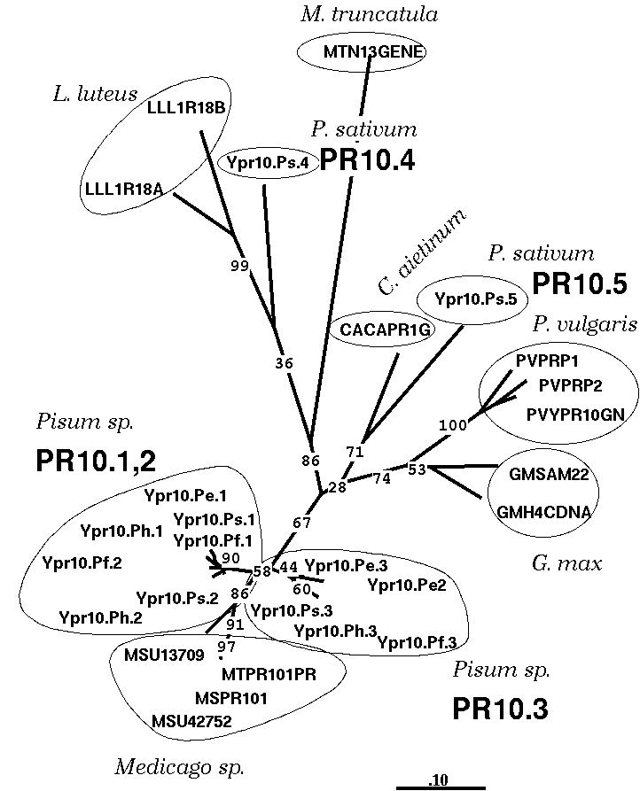
The tree at right shows the relationships of five members of the pathogenesis-related protein family PR10 from legumes.
Numbers at nodes indicate how many replicates a given branch appeared in, out of 100 samples. For example, the branch containing three PR10.5 genes in Phaseolus vulgaris occurs in 100% of the replicate samples. In contrast, the P. sativum PR10.4 gene Ypr10.Ps.4 clusters together with the two L. luteus geens only 36% of the time. This branch is therefore less strongly supported by the data.
There is still some uncertainty as to what bootstrap frequencies actually mean. When Felsenstein initially proposed using bootstrap replicates for evaluating phylogenies, he stated that the bootstrap value, out of 100 trials, was a direct estimator of statistical significance. That is, a branch occurring 95 out of 100 times would be significant at the 5% level. However, the fact that bootstrap samples actually represent a subset of the total data suggests that this is conservatively high. Simulations have shown that "bootstrap values greater than 70% correspond to a probability greater than 95%" (See Hershkovitz and Leipe for reference.)
While it may therefore be difficult to assign cutoff levels for significance to specific bootstrap values, bootstrapping can at least be thought of as a way of showing relative strengths of branches in a given tree.
| PLNT4610/PLNT7690
Bioinformatics Lecture 7, part 3 of 4 |