PLNT4610/PLNT7690 Bioinformatics
Lecture 7, part 2 of 4

B. Methods for tree building -Distance methods

Before discussing common tree building methods, it is instructive to consider the possibility of simply building all possible trees and choosing the best one. For n sequences, the number of possible tree topologies is given in the table. This function increases faster than n-factorial.

# of sequences n	# of trees
3	1
4	3
5	15
6	105
7	945
8	10,395
9	135,135
10	2,027,025
50	2.8 x 10⁷⁴

$∏{}_{i}^{n}$ - the product of function from i to n

For comparison, an estimate of the number of protons in the universe is between 10⁷⁸ and 10⁸².

All 15 tree topologies for 5 species

redrawn from Felsenstein [http://www.cs.washington.edu/education/courses/590bi/98wi/ppt15/sld011.htm ].

Therefore, unless only a small number of sequences are to be included in a tree, methods to avoid considering obviously suboptimal trees must be used to reduce the total number of trees considered.

A phylogenetic tree is a graph consisting of nodes and branches

node - the point at which two branches are joined
branch - the interval between any pair of nodes. Nodes which have no branch point are referred to as terminal nodes.

Any phylogenetic tree can be defined by two components: topology and branch length.

topology - the order in which branches are joined
branch length - the distance between the two nodes of a branch (eg. number of mutations)

There are two main categories of phylogeny methods:

Distance methods - the first step is to calculate a matrix of all pairwise differences between a set of sequences. Next, the tree is constructed to minimize the distance when all branches are added together. Distance methods do not attempt to consider internal branches of the trees, and therefore are not strictly modeled on evolution.
Character methods attempt to reconstruct ancestral nodes of trees in order to fit the tree to an evolutionary model. They therefore use more of the information in the data, at the expense of longer execution time. Character methods include parsimony, maximum likelihood and Bayesean methods.

1. Distance matrix methods

Calculation of distance matrices

In general, DNA distance matrices are calculated such that each mismatch between two sequences adds to the distance, and each identity subtracts from the distance. Scoring matrices include values for all possible substitutions.

General substitution matrix
	A	C	G	T
A	-(a1+a2+a3)	a1	a2	a3
C	a4	-(a4+a5+a6)	a5	a6
G	a7	a8	-(a7+a8+a9)	a9
T	a10	a11	a12	-(a10+a11+a12

DNA scoring methods: (for in-depth descriptions, see http://home.cc.umanitoba.ca/~psgendb/doc/Phylip/dnadist.html)

Jukes and Cantor - all possible nucleotide substitutions are of equal value.
2-parameter method of Kimura - assigns different weights to transitions and transversions.Typically, transversions are weighted as contributing twice the distance of transitions, since transitions occur more frequently.
Maximum likelihood (F84) - assigns distances based on the Kimura formulae, but weighted according to the probabilities of each possible substitution, as determined from nucleotide frequencies.

transition - purine for purine or pyrimidine for pyrimidine substitution

eg. A -> G, G -> A, C -> T, T -> C

transversion - purine for pyrimidine, or pyrimidine for purine substitution

eg. A -> C, A -> T, T -> G, T ->A, C -> G, C -> A etc...

Transitions occur much more frequently during evolution than transversions.

Protein scoring methods (for in-depth descriptions, see http://home.cc.umanitoba.ca/~psgendb/doc/Phylip/protdist.html)
Because of the many nuances in working with proteins, there are many scoring schemes. Most are based on existing PAM or BLOSUM matrices. One common method is to use Dayhoff's PAM 001 matrix to score distances. (One PAM unit is defined as the amount of sequence divergence corresponding to a 1% amino acid replacement rate.) Alternatively, Kimura's protein distance metric simply uses observed amino acid frequencies from a protein to approximate a PAM distance:

D = -ln (1 - p - 0.2 p²)

where p is the fraction of amino acids that differ between two sequences

Using the appropriate scoring methods, all pairwise distances between sequences are calculated. For more details on protein scoring matrices, see the documentation for the Phylip protdist program.

For example, the PHYLIP documentation gives the example of a set of 5 short aligned DNA sequences

Alpha        AACGTGGCCACAT
Beta         ..G..C......C
Gamma        C.GT.C......A
Delta        G.GA.TT..G.C.
Epsilon      G.GA.CT..G.CC

The corresponding distance matrix using the Kimura 2 parameter model is

	Alpha	Beta	Gamma	Delta	Epsilon
Alpha		0.2997	0.7820	1.1716	1.4617
Beta			0.3219	0.8997	0.5653
Gamma				1.4481	1.0726
Delta					0.1679
Epsilon

The Neighbor-Joining method (NJ)

The Neighbor -Joining method is one of the simplest distance methods. It begins by choosing the two most closely-related sequences, and then adding the next most distant sequence as a third branch to the tree. Fitch and Margoliash give a simple example for a tree with 3 sequences A,B and C and the distances between nodes x, y and z:

B C

A 24 28

B
32

Simultaneous linear equations can be used to calculate the branch lengths:

A to B: x + y = 24
A to C: x + z = 28
B to C: y + z = 32

Thus with 3 equations and 3 unknowns we can calculate that x = 10, y = 14 and z = 18. These pairwise distances are the shortest distance between each possible pair of nodes.

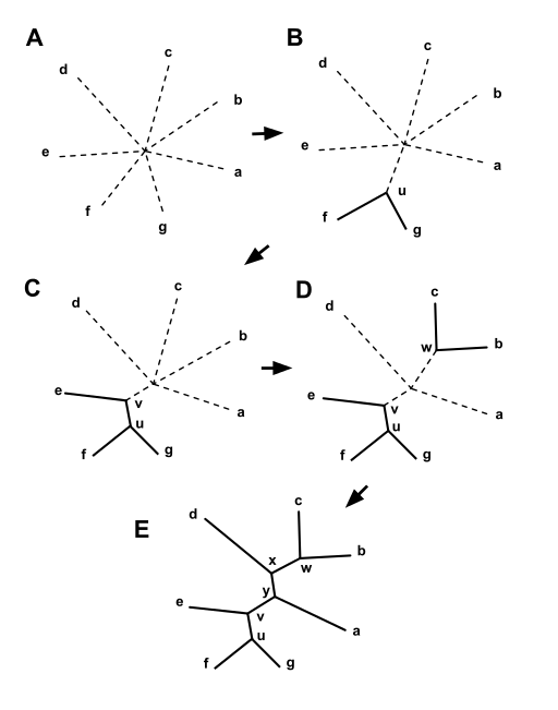
Addition of branches is iterative. Branches are added until all sequences are included in the tree. This is illustrated in the example below:

Starting with a star tree (A), the Q matrix is calculated and used to choose a pair of nodes for joining, in this case f and g. These are joined to a newly created node, u, as shown in (B). The part of the tree shown as solid lines is now fixed and will not be changed in subsequent joining steps. The distances from node u to the nodes a-e are computed from equation (3). This process is then repeated, using a matrix of just the distances between the nodes, a,b,c,d,e, and u, and a Q matrix derived from it. In this case u and e are joined to the newly created v, as shown in (C). Two more iterations lead first to (D), and then to (E), at which point the algorithm is done, as the tree is fully resolved.

from https://en.wikipedia.org/wiki/Neighbor_joining

Advantages

fastest tree building method (scales linearly with the number of sequences)
can use empirical substitution scoring methods

Disadvantages

tests only a single tree
does not consider intermediate ancestors, meaning that there is no requirement for an internally-consistent evolutionary model
misses homoplasies, especially over long distances; long evolutionary distances will be underestimated.

You can learn more about the details of the NJ method at:

Saitou N, Nei M (1987) The neighbor-joining method: a new method for reconstructing phylogenetic trees. Mol. Biol. Evol. 4:406-25.

The Neighbor-Joining Algorithm https://youtu.be/Y0QWFFWQzds

Neighbor joining https://en.wikipedia.org/wiki/Neighbor_joining

The Fitch/Margoliash Least Squares Method

The Neighbor-Joining method only attempts to build one tree. However, the raw pairwise distances are never additive. The ideal example shown above was internally consistent. In the example, the sums of the 3 simultaneous equations (ie. 2 x the sums of the branch lengths) were precisely equal to the sums of the pairwise distances. This will not always be true for real data. In part this is due to undetected homoplasy.

Fitch and Margoliash showed that different sets of internal branch lengths could be obtained by considering alternate trees which moved one or more branches to different parts of the tree. Consider a distance matrix for four sequences with pairwise distances D_ij;

Observed distances D_ij
	A	B	C	D
A	0	0.16	0.38	1.18
B	0.16	0	0.49	0.93
C	0.38	0.49	0	0.91
D	1.18	0.93	0.91	0

The Neighbor-Joining tree for these sequences is

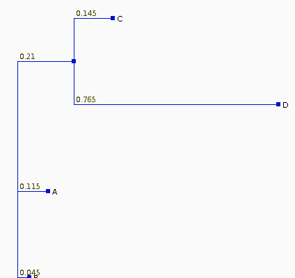
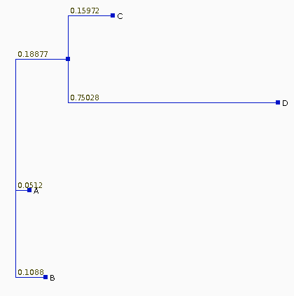
If we recalculate the pairwise distances d_ij from the tree, they are different from the original distances, as shown at right.

The least squares method of Fitch and Margoliash tries different tree topologies, swapping branches among closely-related sequences, and reculating the distances. For each tree considered, a different matrix of distances will be generated (d_ij). The best tree is defined as that tree which minimizes:

Distances recomputed from the tree d_ij
	A	B	C	D
A	0	0.16	0.47	1.09
B	0.16	0	0.40	1.02
C	0.47	0.40	0	0.91
D	1.09	1.02	0.91	0

The Fitch-Margoliash tree for the same distance matrix is

In this simple example, the topologies of the two trees are the same, but the branch lengths of the Fitch tree is a more reliable estimate of the branch lengths.

Advantages

tests more than one tree
still pretty fast
can use empirical substitution scoring methods
global optimization of tree by statistical criteria

Disadvantages

Requires longer execution time than Neighbor Joining, but still quite practical on most computers, for most datasets.
does not consider intermediate ancestors, meaning that there is no requirement for an internally-consistent evolutionary model
misses homoplasies, especially over long distances; long evolutionary distances will be underestimated.

What about UPGMA?

It has been exhaustively demonstrated in the literature, both on theoretical grounds and from phylogenies constructed on strains of known pedigree, that UPGMA is the least robust method. It is based on the assumption that rates of evolution are constant along all branches ie. follows an evolutionary clock. This assumption is almost never valid. Especially with the many choices of far more sophisticated phylogeny inference methods, there is little justification for ever using UPGMA.

One point to make is that a comparison of Neighbor-Joining results with UPGMA results could provide a test for the hypothesis that evolution in a given tree is clock-like.

As well, UPGMA might be useful for constructing trees where no underlying evolutionary model is assumed. For example, in clustering of genes into groups based on similarities in gene expression patterns, it would be incorrect to assume that genes with similar patterns of expression must in some sense be related in an evolutionary sense.

Distance Methods [http://helix.biology.mcmaster.ca/721/outline2/node49.html]
Nei M and Roychoudhury AK (1993) Evolutionary Relationships of Human Populations on Global Scale. Mol. Biol. Evol. 10:927-943.
Saitou N, Nei M (1987) The neighbor-joining method: a new method for reconstructing phylogenetic trees. Mol. Biol. Evol. 4:406-425.

last page

PLNT4610/PLNT7690 Bioinformatics
Lecture 7, part 2 of 4