last  page

PLNT4610/PLNT7690 Bioinformatics Lecture 11, part 1 of 1

next page

A. OVERVIEW

B. Impact of the quality of the assembly on annotation

C. Repeat identification and masking

D. Similarity based alignment of protein and RNA sequences to coding regions

E. Prediction of gene structure

F. GFF3 Genome Annotation format

A. Overview

The goal of genome annotation is to identify features found in a genome, including coding sequences for proteins and RNAs, repetitive elements and a spectrum of other types of information found in genomes. The end product is an annotated genome, as represented by an entry in the GenBank database.

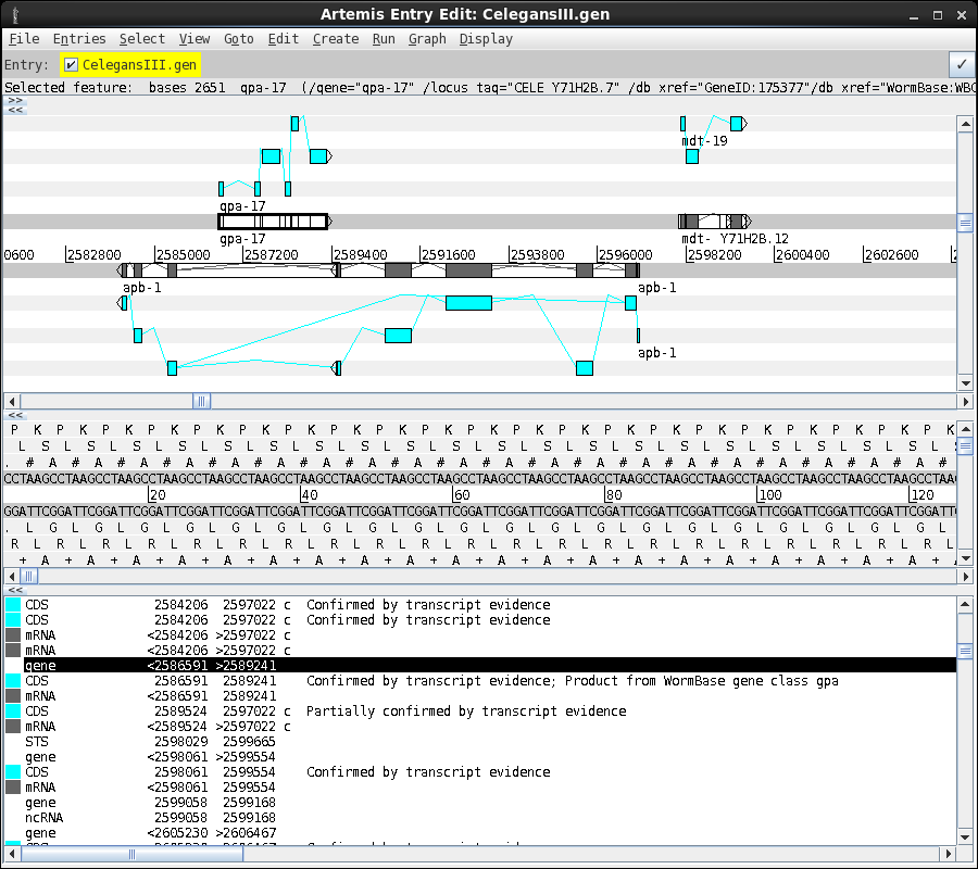
An example of an annotated genome is shown below. A region of the C. elegans chromosome III is shown in the artemis viewer. Note that two genes are shown on the forward strand, and a single gene on the reverse strand. The lower panel gives the text annotation corresponding to features shown in the viewer.

Genome annotation is best described as a pipeline of steps. The example at right shows the NCBI eukaryotic genome annotation pipeline, which combines information for several sources, when available. These include the RefSeq genes and mRNA data, known protein sequences, as well as RNA seq data, if available. Coding regions are found through simple BLAST searches. The coding regions are more precisely annotated using ab initio gene prediction software to produce gene models. Gene models include precise locations of exon/intron boundaries, as inferred from mRNA or EST data.

from https://www.ncbi.nlm.nih.gov/genome/annotation_euk/process/

B. Impact of the quality of the assembly on annotation

As with everything else, the quality of the starting material is the single most important factor determining the results. A low quality genome will give low quality gene calls. Two parameters that can indicate whether a genome is worth annotating are N50 and percent coverage.

N50 - N50 is the median contig size, such that 50% of the contigs are larger than N50, and 50% are smaller. It makes sense that if N50 contig sizes are smaller than the size of genes, then most genes would be broken between two or more contigs. Therefore, one guideline for a quality assembly is to have contigs larger than the median size of genes. Figure 1 shows a direct relationship between genome size and the median size of a gene. In terms of successful genome annotation, we need larger contigs for large eukaryotic genomes than we do for prokaryotic genomes.

Fig. 1 from Yandell and Ence

Note in the above figure that plant genes don't seem to follow this linear relationship. Over 2 logs of genome size, gene size increases maybe by 10%.

percent coverage - The percentage of the genome covered by an assembly. If genome size, as estimated from the assembly is close to the actual genome size, then most genes will probably be found, especially where the number of scaffolds is not large. Not getting the entire genome may still not be a problem in eukaryotic genomes with lots of repetitive sequences. The repetitive fraction of a genome tends to be underestimated in incomplete genome assemblies, because repetitive sequences often prevent the assembly of larger contigs.

completeness of transcriptome - Not all mRNAs are expressed in all tissues. Since transcripts from the transcriptome are part of the annotation process, many genes could be missed if they are not present in one or more of the tissues, developmental stages or conditions used in assembly of the transcriptome.

C. Repeat identification and masking

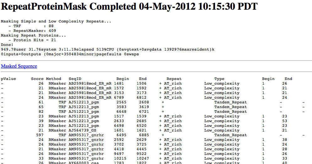
Because much of the annotation process relies upon similarity comparisons, it is critical to mask repeats within your genomic sequences. Two types of repeats need to be masked:

• short tandem repeats (low complexity repeats such as satellite DNA)
• repetitive elements - repetitive sequences such as transposons that can make up large percentages of genomes.

• soft masking - conversion of repeats into lowercase nucleotides
  
• hard masking - conversion of repeats into N's
  

Many programs for similarity searches, such as BLAST and FASTA, will ignore masked sequences in both queries and databases.

For repetitive elements, repeat masking programs require a database of known repeats to be masked. These are easily available for model genomes. However, for most genomes, you would need to create your own database of repetitive elements to be masked.


from http://eagle.fish.washington.edu/trilobite/sr320_labnotebook_060113.enex/TGAGA%20cg_alpha0.3.2%20Repeat%20Masker.html

Repeat masking is actually part of genome annotation, since the output from repeat masking programs can be used to annotate the location of known repetitive elements in genome.

D. Similarity based alignment of protein and RNA sequences to coding regions

This step amounts to the discovery of protein coding regions, often annotated as CDS regions.

Similarity search programs such as BLASTX can compare a genomic nucleotide sequence with a protein database to find potential coding regions. In the example at right, output for a 9.5 kb contig from a fungal genome shows three potential coding regions. The right most coding region appears to include an intron between two CDS regions.

E. Prediction of gene models

Similarity alignment results only give the approximate locations of CDS features. The precise exon/intron structure of a gene, along with other features such as ribosome binding sites, 5'UTRs, 3'UTRs or promoter regions, require more sophisticated gene prediction tools. The goal is to create a model of a gene describing these features with precise begin and end points.

For example, splice junctions are predicted using tools such as splign. Splign predicts exon/intron structure based on cDNA/EST sequences found in genome databases. Splign works in three steps:

1. local alignment - performs a standard Smith-Waterman alignment between a set of cDNA sequences and the genomic sequence
2.  alignments are used to identify the location of each cDNA in the genomic data
3. an optimal alignment is performed on the cDNAs and the genomic data, using a splice site prediction model.

In the example, the sequence of an exon boxed in green is shown. The cDNA is on top (pink) and the chromosomal sequence is on the bottom (blue). The AG of the splice acceptor 5' to exon 5, and the GT of the donor 3' to exon 5 are highlighted in green.

from https://www.ncbi.nlm.nih.gov/Web/Newsltr/V14N2/splign.html

Annotation pipelines such as MAKER combine information from many sources, including gene predictors, BLAST, and repeat maskers, to create integrated alignments. At right is an gene model, viewed in the Apollo genome viewer.

from http://gmod.org/wiki/MAKER

F. GFF3 Genome Annotation format

 0  ##gff-version   3
 1  ##sequence-region   ctg123 1 1497228       
 2  ctg123 . gene            1000  9000  .  +  .  ID=gene00001;Name=EDEN
 3  ctg123 . TF_binding_site 1000  1012  .  +  .  ID=tfbs00001;Parent=gene00001

 4  ctg123 . mRNA            1050  9000  .  +  .  ID=mRNA00001;Parent=gene00001;Name=EDEN.1
 5  ctg123 . five_prime_UTR  1050  1200  .  +  .  Parent=mRNA0001
 6  ctg123 . CDS             1201  1500  .  +  0  Parent=mRNA0001
 7  ctg123 . CDS             3000  3902  .  +  0  Parent=mRNA0001
 8  ctg123 . CDS             5000  5500  .  +  0  Parent=mRNA0001
 9  ctg123 . CDS             7000  7600  .  +  0  Parent=mRNA0001
10  ctg123 . three_prime_UTR 7601  9000  .  +  .  Parent=mRNA0001

11  ctg123 . mRNA            1050  9000  .  +  .  ID=mRNA00002;Parent=gene00001;Name=EDEN.2
12  ctg123 . five_prime_UTR  1050  1200  .  +  .  Parent=mRNA0002
13  ctg123 . CDS             1201  1500  .  +  0  Parent=mRNA0002
14  ctg123 . CDS             5000  5500  .  +  0  Parent=mRNA0002
15  ctg123 . CDS	     7000  7600	 .  +  0  Parent=mRNA0002
16  ctg123 . three_prime_UTR 7601  9000	 .  +  .  Parent=mRNA0002

17  ctg123 . mRNA            1300  9000  .  +  .  ID=mRNA00003;Parent=gene00001;Name=EDEN.3
18  ctg123 . five_prime_UTR  1300  1500	 .  +  .  Parent=mRNA0003
19  ctg123 . five_prime_UTR  3000  3300	 .  +  .  Parent=mRNA0003
20  ctg123 . CDS             3301  3902  .  +  0  Parent=mRNA0003
21  ctg123 . CDS	     5000  5500	 .  +  2  Parent=mRNA0003
22  ctg123 . CDS	     7000  7600	 .  +  2  Parent=mRNA0003
23  ctg123 . three_prime_UTR 7601  9000	 .  +  .  Parent=mRNA0003

from http://rice.bio.indiana.edu:7082/annot/gff3.html

Unless otherwise cited or referenced, all content on this page is licensed under the Creative Commons License Attribution Share-Alike 2.5 Canada

last  page

PLNT4610/PLNT7690 Bioinformatics Lecture 11, part 1 of 1

next page