previous  page PLNT4610/PLNT7690 Bioinformatics
Lecture 12, part 3 of 3
first page

D. Transcriptomic Data pipelines

1. de-novo assemblies and read mapping

The first step in the data pipeline aligns sequencing reads, either by mapping each read to a gene, or by de-novo assembly of transcripts from the reads themselves.


from Thiru, P RNA-seq: Methods and Applications. http://jura.wi.mit.edu/bio/education/hot_topics/RNAseq/RNA_Seq.pdf

Mapping transcripts is generally easier in prokaryotes, and requires less computational time, than in eukaryotes. Mapping transcripts to reads is more complicated for eukaryotes, for a variety of reasons.

Prokaryotes
Eukaryotes
smaller genomes and fewer genes much larger genomes and more genes
more likely to have completely sequenced and annotated genomes less likely to have completely sequenced and annotated genome
almost all genes present in single copies many genes are in multigene familes
genes seldom have introns genes almost always have introns; many genes have splice variants
haploid
genomes may be polyploid


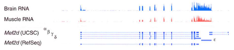
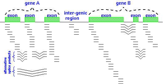
The illustration at right shows RNA-seq reads aligned to two eukaryotic genes A and B. Reads that span part of an exon are shown as single lines, whereas reads that include parts of two adjacent exons are indicated by V-shaped lines. The presence of introns being spliced out of pre-mRNA transcripts means that alignment programs have to check to see whether a read contains part of the 3' end of one exon and part of a 5' end of another exon.

It is also notable that most transcriptomics experiments contain reads that map in presumably non-coding intergenic regions. These can either indicate that there are previously-unannotated transcribed regions in the genome, or the presence of untranscribed pseudogenes.

Transcriptomics is also revealing that alternative spllicing occurs more frequently in eukaryotic gene expression than was previously appreciated.

Implementation of a gene expression pipeline

There is no such thing as an off-the shelf pipeline that can simply take raw reads, allow you to press a button, and generate a complete differential expression profile. This is in part because the nature of RNA-seq analysis is such that each step in the process is a decision point at which the results should be inspected to decide both whether the previous step needs to be re-run with different conditions, or with a different program, and also to decide, based on the result of the previous step, which program to use in the next step, or which parameters.
A second reason is that both the RNA sequencing technologies, and the bioinformatics tools are always changing to incorporate new advances. Therefore, RNA analysis pipelines will always be a work in progress.
The main steps can be summarized as follows:

For teaching purposes, this lecture will use as an example the RNA seq pipeline currently in place at the Bio Information Technologies Lab at the University of Manitoba.

Pre-processing 
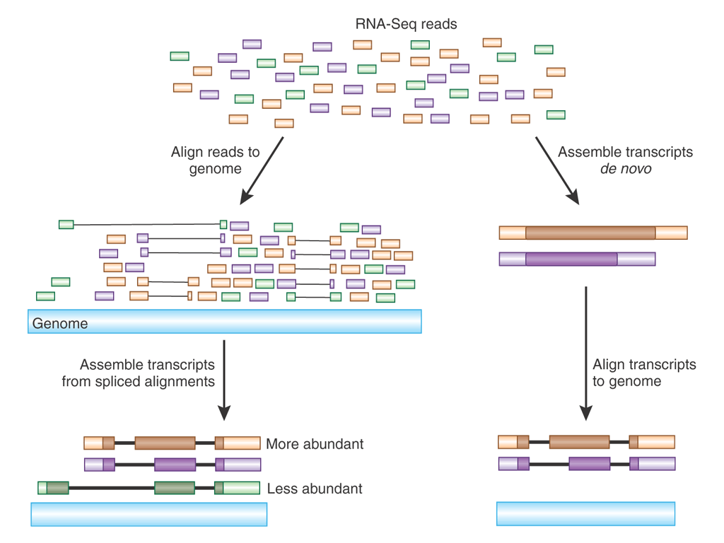
and assembly of reads

A simplified workflow for transcriptome assembly is shown at right.

Transcriptome assembly is carried out within the transcriptome directory, and for each major step, a separate subdirectory is used.

Raw read files are saved in the reads directory, and symbolic links to these files, with short, meaningful names, are created.

Sequencing adaptors are removed from the raw reads by Trimmomatic and the files containing the trimmed reads are saved in reads.Trimmomatic.

The trimmed reads are used as input by Rcorrector, which corrects errors in the reads and writes the corrected reads to the reads.Trimmomatic.Rcorrector directory.

At each step, FASTQC is run to check the properties of the reads.

Finally, the assembly itself is done using programs such as Trinity  which produces contig files and scaffold files. For each assembly, transrate produces a reports with extensive statistics that can guide the choice of which assembly is best, or which assemblies should be repeated with different a parameters for improvement.


Correction of RNAseq reads is complicated by the dependence of k-mer frequencies on the level of RNA transcripts.

Read correction programs like Quake or Pollux correct DNA sequencing reads by assuming that all reads, and therefore all k-mers, should be present in roughly even quantities for a genome with adequate coverage.

By definition, RNAseq has the goal of measuring the level of RNA transcripts, based on the frequencies of reads from each gene. For this reason, k-mers from strongly expressed transcripts are expected to be found in higher numbers than k-mers from weakly expressed transcripts. It would therefore not be valid to correct RNAseq reads using programs designed for correction of genome sequencing reads.

However, we can expect that k-mer frequencies derived from any particular transcript (gene) should be at even levels. In other words, for a strongly expressed gene A, all k-mers from that gene should be seen at a frequency of kA, while for a weakly expressed gene B, the frequencies of k-mers for gene B should be seen at a frequency of kB.

Rcorrector corrects reads using only k-mers occurring at similar frequencies. In one sense, the requirement for similar k-mer frequencies within a transcript adds some reliability to the correction, by constraining the possible solutions to the correction problem.

WARNING!  Do not use DNA read correction programs to correct RNA reads.

DNA read correction programs like pollux assume equal k-mer frequencies for all k-mers.
RNA read correction programs like Rcorrector require that k-mer frequencies are similar within a transcript, but recognize that because each transcript occurs at a different level, each transcript will have different k-mer frequencies. Strongly expressed transcripts will have high k-mer frequencies, while weakly expressed transcripts will have low k-mer frequencies.


Generation of gene expression data
Note: For many years, the Tuxedo pipeline, consisting of TopHat, Bowtie, Cufflinks and Cuffdiff was widely used for generating differential expression data from reads.  The authors of Tuxedo have released a new package called Ballgown, which supersedes those programs.
Pertea M, Kim D, Gertea GM, Leek JT, Salzberg SL (2016) Transcript-level expression analysis of RNA-seq experiments with HISAT, StringTie and Ballgown. Nature Protocols 11:1650. doi:10.1038/nprot.2016.095.


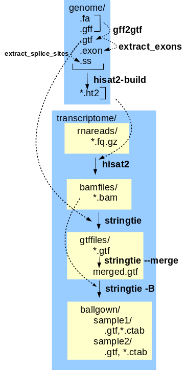
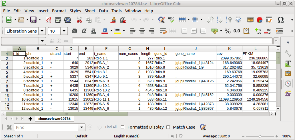
The final transcriptome assembly can now be used to generate gene expression data from the corrected reads. This tutorial implements the  Hisat, Stringtie, Ballgown gene expression pipeline.

Hisat-build creates files that index the features in the annotated genome, so that reads can be mapped to features.   Mapped reads are written to .bam files.

For each read file, hisat2 maps reads to the genome. Next, stringtie assembles the reads into transcripts, including alternative splicing products. Transcripts mapped to genomic locations are written to .gtf files.

Transcripts from all sets of reads are merged into a single .gtf file by stringtie --merge.

The final step is to generate tables of gene expression values. stringtie -B reads the mapped reads from the .bam files and the mapped transcripts from the .gtf files, and writes tables of FPKM values to comma-separated value files that can be read by the BioConductor R package for further analysis.


2. Normalization

As shown in the illustration above, more reads will be found for larger genes than for smaller genes. Consequently, it is necessary to correct gene expression levels for the size of each gene. To make results comparable across experiments, we also need to correct for the number of reads or fragments that were mapped to a gene in the genome or transcriptome.
Depending on whether you are doing single reads or paired-end reads, there are two almost identical formulae.


RPKM - Reads Per Kilobase of transcript per Million mapped reads

RPKM = C/LN

where
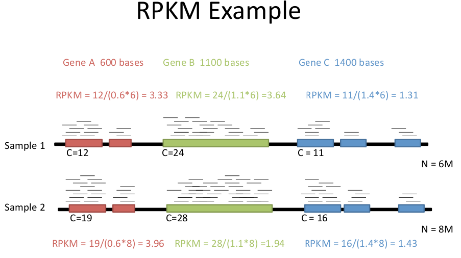
C : number of mappable reads on a feature
L : Length of feature (in kb)
N : Total number of mappable reads (in millions).
    Not all reads can be mapped to a specific gene.


from Thiru, P RNA-seq: Methods and Applications. http://jura.wi.mit.edu/bio/education/hot_topics/RNAseq/RNA_Seq.pdf

FPKM - Fragments Per Kilobase of transcript per Million mapped reads (necessary for paired-end reads)

FPKM = F/LN

where
F : number of mappable fragments on a feature. There are usually two reads for a fragment with paired end reads. Each pair of reads counts as a fragment.
L : Length of feature (in kb)
N : Total number of mappable reads (in millions)

Ballgown creates a file for each set of reads with FPKM values and other statistics for each gene.


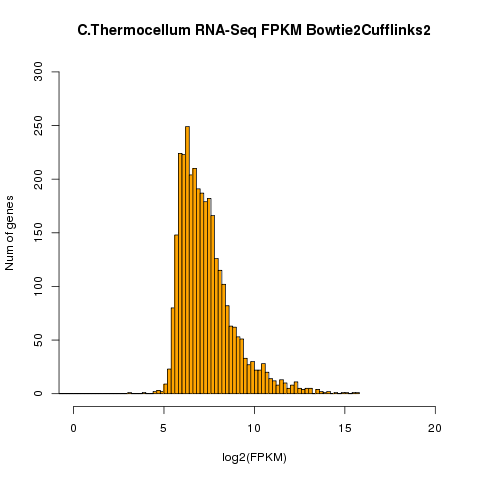
Example of distribution of genes for a given FPKM.

RNAs from Clostridium thermocellum grown in exponential phase culture were assembled in a BowTie-TopHat Cufflinks pipeline.

FPKM is represented as the log2 of FPKM. The number of genes expressed at a given FPKM level are represented as bars on the Y-axis.


3. Which genes show a  "significant" difference between treatments?

Correction for the "Thousands of Genes" problem

With RNAseq, the results for each gene could be considered to be a different experiment. What this means is that if the expression levels of 10,000 genes are compared between two treatments, we expect, when using p= 0.01 as a cutoff for significance, that about 100 genes would appear to have significantly different levels, just by random chance alone!  We need ways to correct p values so that one gets a more realistic estimate of statistical significance, for each gene compared.

Many gene expression programs use statistical methods such as ANOVA to calculate a p value p(x >
α), indicating the probability, the observed value x would exceed α by random chance alone. In many experiments, we accept p values less than 0.05 or 0.01 as being significant. Remember, however, that this means that respectively, 1 out of 20 times, or 1 out of 100 times, we get a false positive! Therefore, the threshold p values for assessing significance must be adjusted. The page linked below presents some of the ways of correcting p values in transcriptomics experiments.

https://physiology.med.cornell.edu/people/banfelder/qbio/resources_2008/1.5_GenespringMTC.pdf

Volcano Plots

Volcano plots let you assess the significant changes, between treatments, for the gene population as a whole
by Natalie Bjorklund, University of Manitoba

Volcano plots are a way to determine if there is data present that is worth taking a further look at. Gene expression experiments are typically designed to compare two things, such as exponential growth phase versus stationary phase, and looking for gene expression levels that change, either going up or down. Also because the experiments are done in replicates it is possible to determine how much variation there is between the replicates and use that value to determine if the change in gene expression is statistically significant or just a result of differences between each experimental replication. The Volcano plot allows you to quickly see if there is any difference that is both large and statistically significant. If the plot does not form a proper looking Volcano plot something is wrong. (Converting the values to log often makes the data fit into the same general order of magnitude and removes issues like different unit values so Volcano plots for gene expression are typically shown in -log10 of the p value and log2 fold change.)

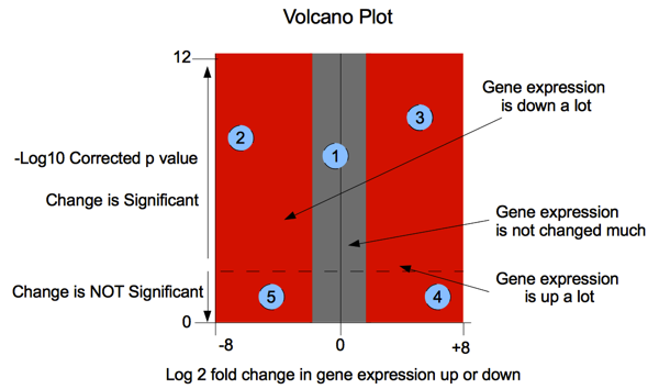
In the diagram below:

Probe 1: a statistically significant result (consistent across the experimental replicates) showing little change in expression.

Probe 2: a large decrease in gene expression that is also statistically significant (replicates match well)

Probe 3: a large increase in gene expression that is also statistically significant, (replicates match well)

Probe 4: a large increase in gene expression but one that is not statistically significant because the replicates of the experiment did not match well ie. observed change is less than the variance between replicates.

Probe 5: a large increase in gene expression but one that is not statistically significant because the replicates of the experiment did not match well


Example of a Volcano Plot showing which genes differ significantly, between two treatments. In this experiment, gene expression levels are compared in two different Clostridium thermocellum strains grown in exponential culture.

4. Differential expression

Ideally for each gene in the genome, RNAseq can give us an expression map, showing the level of expression of each gene, or even each exon (in the case of alternative splicing).


Maps are shown for five alternative transcripts alpha through epsilon, along with the RefSeq map for this gene. Above the maps, the number of mapped reads are shown from RNA in brain and muscle cells.

In principle, the level of expression for each exon in a gene should be identical, since each exon should be present in each mRNA transcript. There are at least three possible reasons why this might not be true:

Examples of Differential Expression

Trapnell, C et al. (2012) Differential gene expression and transcript expression analysis of RNA-seq experiments with TopHat and Cufflinks. Nature Protocols 7:562-578. doi:10.1038/nprot.2012.016.


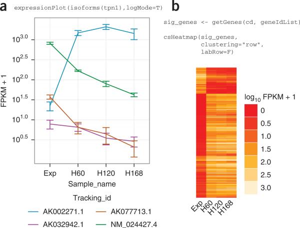
Output from CummeRbund.

a) CummeRbund can generate expression profiles for single genes. In this example, FPKM levels for four different tropomyosin I genes are shown in four different samples, with replicates, at four stages of differentiation in myoblast cells in mouse muscle tissue.

b) Clustering of gene expression in myoblast cells over a differentiation timecourse in mouse muscle tissue.


RNA-Seq makes it possible to compare the expression of different splice variants

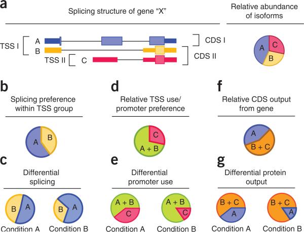
a) Map of a hypothetical gene with two different Transcription Start Sites (TSS) and three splice variants.

b - e)  Detection of variants make it possible to separately examine differential promoter use and differential splicing, in different conditions.

f, g) Since different proteins would also be generated by these splice and transcription variants, the proteome may be affected to


Unless otherwise cited or referenced, all content on this page is licensed under the Creative Commons License Attribution Share-Alike 2.5 Canada

previous  page PLNT4610/PLNT7690 Bioinformatics
Lecture 12, part 3 of 3
first page