PCA: 3D View
(Raychaudhuri et al. 2000)
PCA is used to attribute the overall variability in the data to a reduced set of variables termed principal components. To each principal component a certain fraction of the overall variability of the data is attributed such that each successive component determined accounts for less of the variability than the previous one. This ranks the components in order of decreasing determination of data variability. The first three principal components are used to map each element into a three dimensional viewer.
The option indicates whether to perform the analysis on genes or experiments.
The selection option determines the type of matrix centering (by mean, median, or none) to be performed before the PCA analysis is run
The option determines which algorithm to run when clustering by samples. The complete algorithm creates an nxn distance matrix where n is the number of genes. As data sets get large, memory requirements increase exponentially. For most cases, it is a sufficient approximation to calculate the result using the smaller mxm distance matrix where m is the number of samples. This dramatically decreases memory requirements and calculation time.
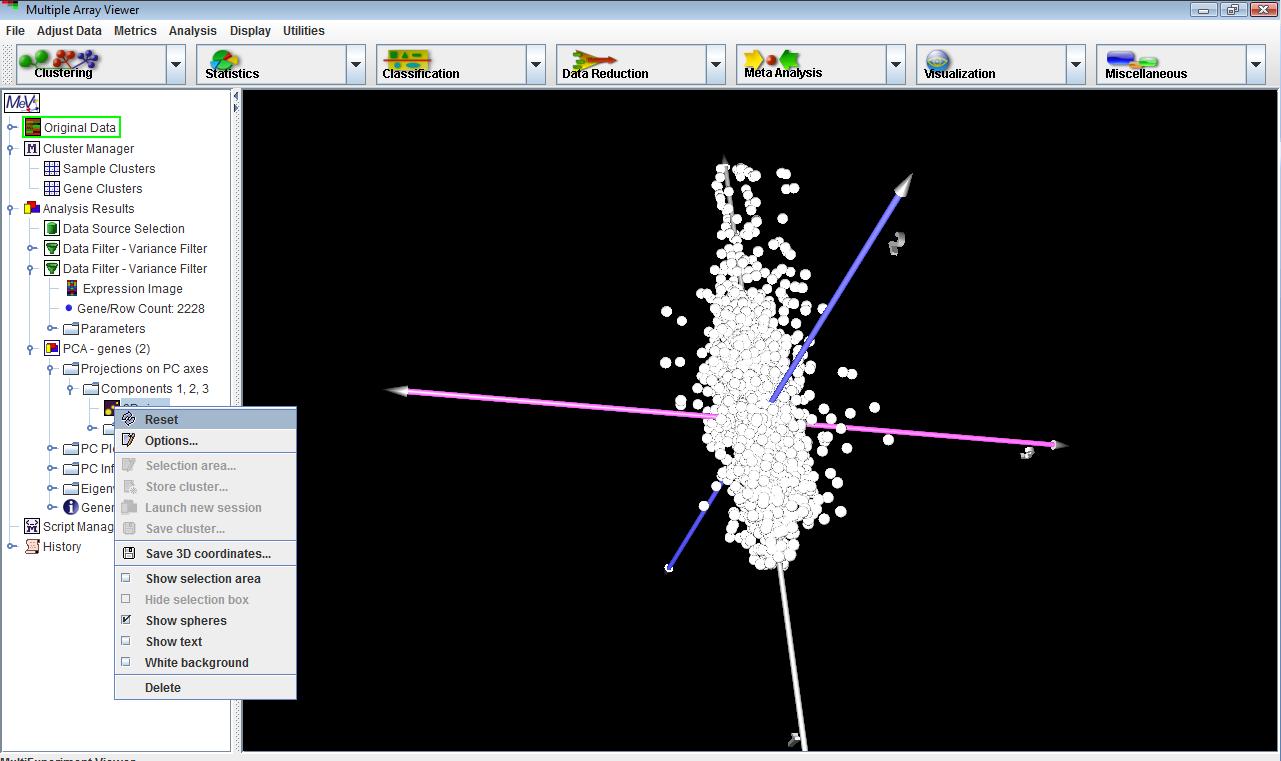
Once the calculations are complete, select the PCA node under Analysis to view the PCA results. Under the node called “Projections on PC Axes” are the default plotting of components 1, 2 and 3. Right-clicking on this node will allow other components to be chosen for plotting. These new plots will show up as new nodes under this node.
The first three (Scale axix X, ...Y, and ...Z) are for scaling the X, Y, and Z axis ranges. The entered value is the viewable distance on either side of the origin.
The floating point value scales the size of each element point in space.
The floating point value scales the size of each element point which has been selected.
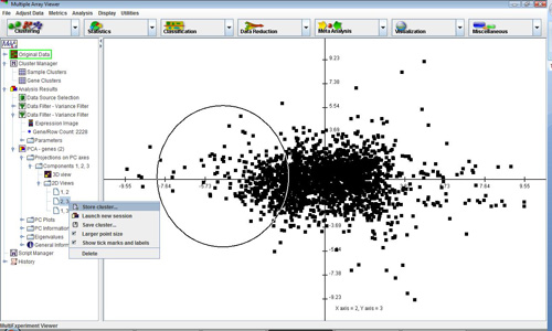
3D view is one of the primary PCA displays, and is a three dimensional view. The display can be rotated and shifted by left dragging or right dragging respectively. Right clicking on the 3D view node will display a popup menu that allows the user to change the 3D view’s display options and create a selection area (essentially a cube) to define a cluster. The 2D views will display plots of any two components at a time.
PC plots, PC information and Eigenvalues detail the calculations behind the construction of the display. Often some meaning such as overall expression level, expression trends, or some other aspect of the data set can be found to correlate to the principal components. Using the PC plots, and noting where clusters of elements showing various trends labeled in other algorithms fall in the 3D viewercan help to assign some tentative meaning to each component. Note that interpretation of the components is not exact and is somewhat subjective.
The first three
The dictate the dimensions of the selection area in 3D space.