TUTORIAL: PHYLOGENETIC ANALYSIS USING DISTANCE METHODS |
June 24, 2021 |
TUTORIAL: PHYLOGENETIC ANALYSIS USING DISTANCE METHODS |
June 24, 2021 |
| The PHYLIP programs are command line
programs, but can be run by BioLegato. The programs in the PHYLIP package are interactive programs designed to be run at the command line. BioLegato can run these programs by generating the keystrokes you would have typed to set program parameters. Construction of a phylogeny using
distance methods involves two steps:
|
In this tutorial, we will demonstrate phylogeny using both
protein and DNA alignments as input.
Start by creating a directory called distance, and save chitIII.pro.mafft.fsn
and chitIII.CDS.pal2nal.fsn
to this directory. Open these files in blpalign and blnalign,
respectively.
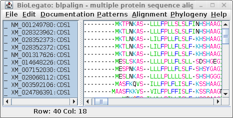
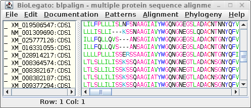
| blpalign - protein
alignment |
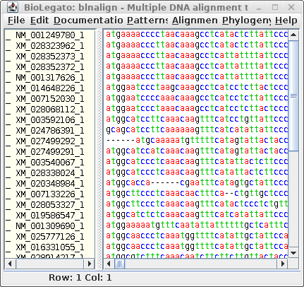
blnalign - DNA alignment |
 |
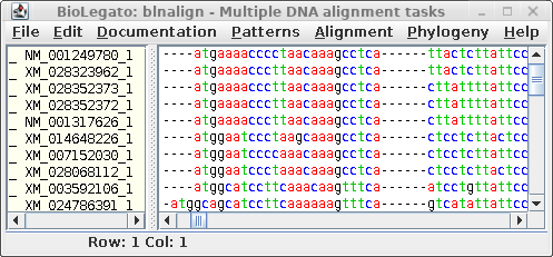 |
For comparison only 10 of the 40 sequences in the alignment are
shown for both proteins and DNA. The alignments have been scrolled
to show a gap of two amino acids (eg. AS--LLL) in the protein,
corresponding to three codons (six gap positions) in the DNA (eg.
gcctca------ttactctta). The N-terminal regions of the proteins
vary in length, which is why gaps are also seen in the N-terminal
region of the alignment.
The other item of note is that ":CDSx" is appended to the
Accession numbers of the proteins (which are actually the
Accession numbers of the GenBank DNA entries from which they were
translated. These CDS labels indicate which CDS from each entry
was used (remember, long DNA sequences may contain many CDS
features). When Ribosome translates proteins, it automatically
shortens the CDSx label to _x, in part because some programs have
limits to the length of sequence names. As we proceed, the _x
naming convention will be used.
| Why compare DNA and
protein phylogenies? Due to the degeneracy of the genetic code, DNA alignments contain evolutionary information that is lost from protein alignments. In principle then, more realistic phylogenetic trees should be obtained from DNA alignments. The problem is that the small alphabet size (n=4) of DNA, compared to the alphabet size of proteins (n=20) means that alignment of proteins, especially where multiple gaps are found. The solution as shown above is to align the proteins, and then align the DNA sequences to the protein alignment. In effect, this preserves evolutionary information that would otherwise be hidden in the protein alignment. In practice, it is a good idea to do phylogenies on both proteins and DNA sequences. |
The whole point of using multiple sequence alignment as input for phylogeny programs is that over the course of evolution, insertions and deletions (indels) occur in genes. Multiple alignments insert gaps into sequences to make amino acids at homologous positions to line up.
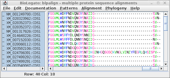
| At right we see the alignment scrolled to the
C-terminal region. It is obvious that an insertion of 29
amino acids occurred in XM_024786391, which we can assume
was a recent event since this insertion was not seen in any
of the other sequences. A problem arises because phylogeny programs treat each position (column) independently. That is, the gap would be treated as if it was 29 independent indels, resulting in an artificially long branch on the tree, separating XM_024786391 from all other sequences. |
 |
The other problem with gappy regions is that they are usually regions in which any multiple alignment is less reliable, because it is not always obvious where gaps should be inserted.
One common solution to this problem is to edit out ALL positions
containing gaps. The downside of this approach is that indels are
highly informative from an evolutionary standpoint, because a
single indel, regardless of its size, can point to ancient events
which instruct the deeper branches of phylogenetic trees. In other
words, completely eliminating all gap positions would be throwing
away useful data.
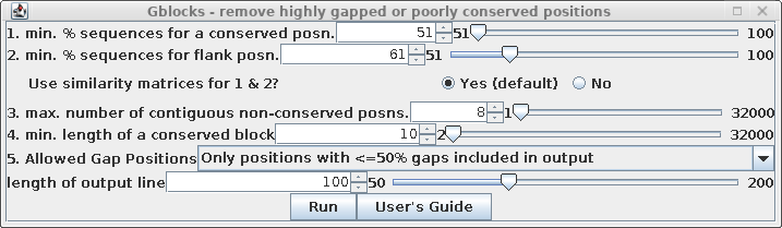
Gblocks from the Castresana lab gives us a more sophisticated way
to "trim" gaps, while retaining some gap positions.
To create a de-gapped alignment, select all sequences in the
protein alignment and choose Alignment --> Gblocks.
| Set "Allowed Gap positions" to "Only
positions with <= 50% gaps. This will retain some gap
positions, as we'll see below. See the Gblocks documentation
for more detailed information on fine-tuning gappy regions
in multiple alignments. |
 |
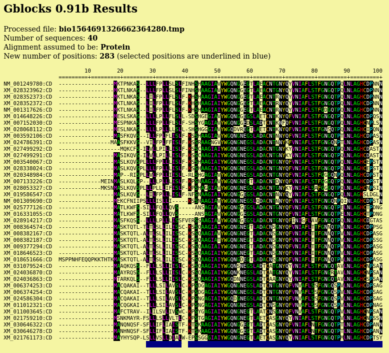
| Output pops up in a new blpalign window. This
output was saved in chitIII.pro.maaft.gblocks.fsa. One of the strong points of Gblocks is the HTML output, excerpted below. The first 100 positions of the alignment, out of 352 positions are shown. Conserved amino acids are highlighted. Based on setting for conserved blocks and flanking posiitons, a subset of 283 positions (underlined in blue) were extracted from the alignment into the blpalign window at right. |
 |
| Next, let's run Gblocks on the DNA alignment
in blnalign. Save this output in chitIII.CDS.pal2nal.gblocks.fsn. (The HTML output for the DNA alignment is not shown.) |
 |
| For routine distance tree construction, the method of Fitch and Margoliash is the method of choice. FITCH allows for variable rates of evolution in different lineages, and iterates the tree to minimize the least squares distance across the entire tree. Although Neighbor-Joining is faster, it is also much less thorough, only considering one tree. It is probably the least rigorous method for constructing a phylogeny . Go to the DNA alignment in blnalign and choose Edit --> Select All. Next choose Phylogeny --> DNA Distance methods. Choose the Fitch-Margoliash method. | 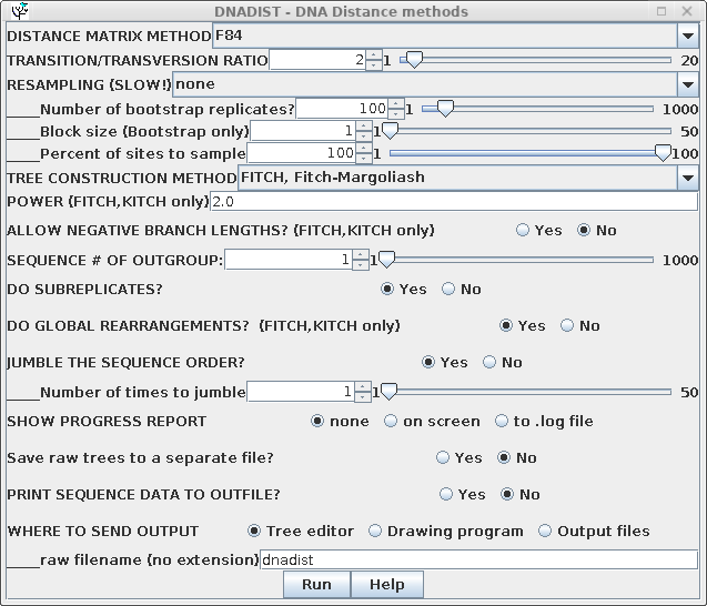 |
DNADIST will calculate a distance matrix, and then FITCH will run, and by default, 3 windows will appear
OUTFILE- the report on the
phylogeny
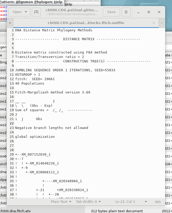
TREEFILE - the machine -readable
treefile. Readable by programs such as DRAWTREE, DRAWGRAM, and
Archaeopteryx.
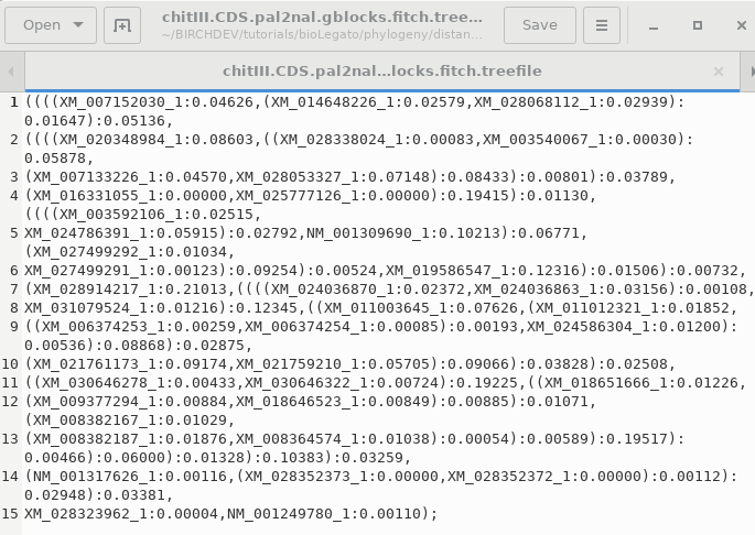
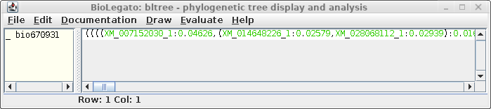
The treefile also pops up on a bltree window, allowing further
tasks to be performed using the tree as input.
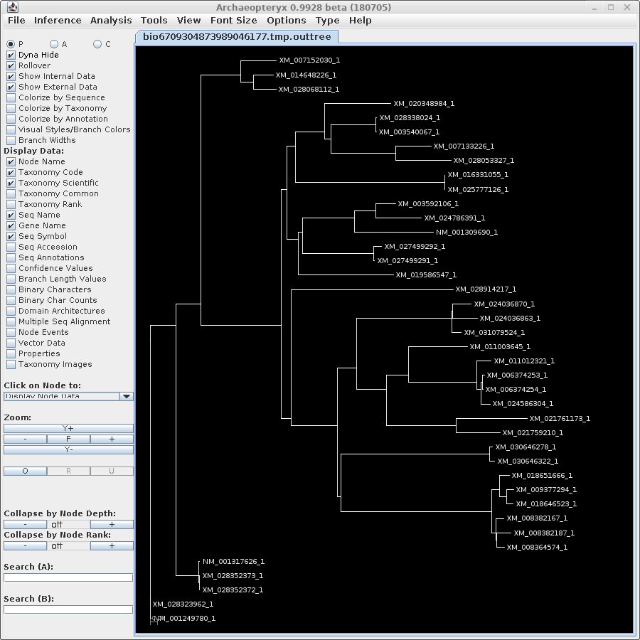
TREEFILE - the treefile in the Archaeopteryx tree
editor.
|
Note: Do NOT save the contents of the Archaeopteryx
window using the .treefile extension. You will overwrite
the original treefile. Archaeopteryx saves files in
phyloXML format with the extension ".phyloxml". |
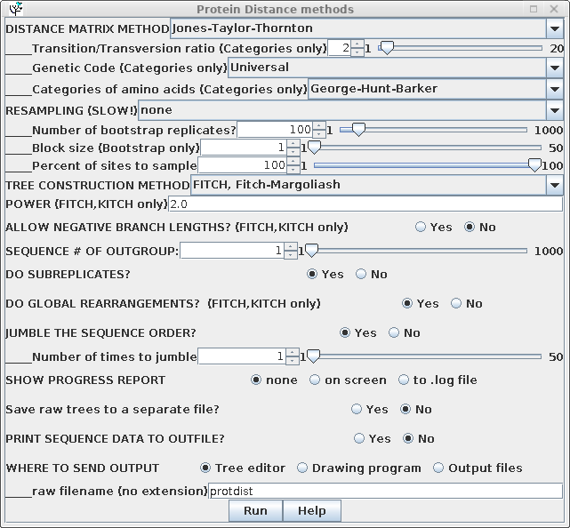
| Some of the parameters for construction of
the distance matrix using PROTDIST are different from those
for DNADIST. These include several different methods
for constructing distance matrices, as well as a choice of
alternative genetic codes, where appropriate. Once the distance matrix is constructed, there is no difference in computation of the phylogenetic tree, so all parameters are the same as previously. |
 |
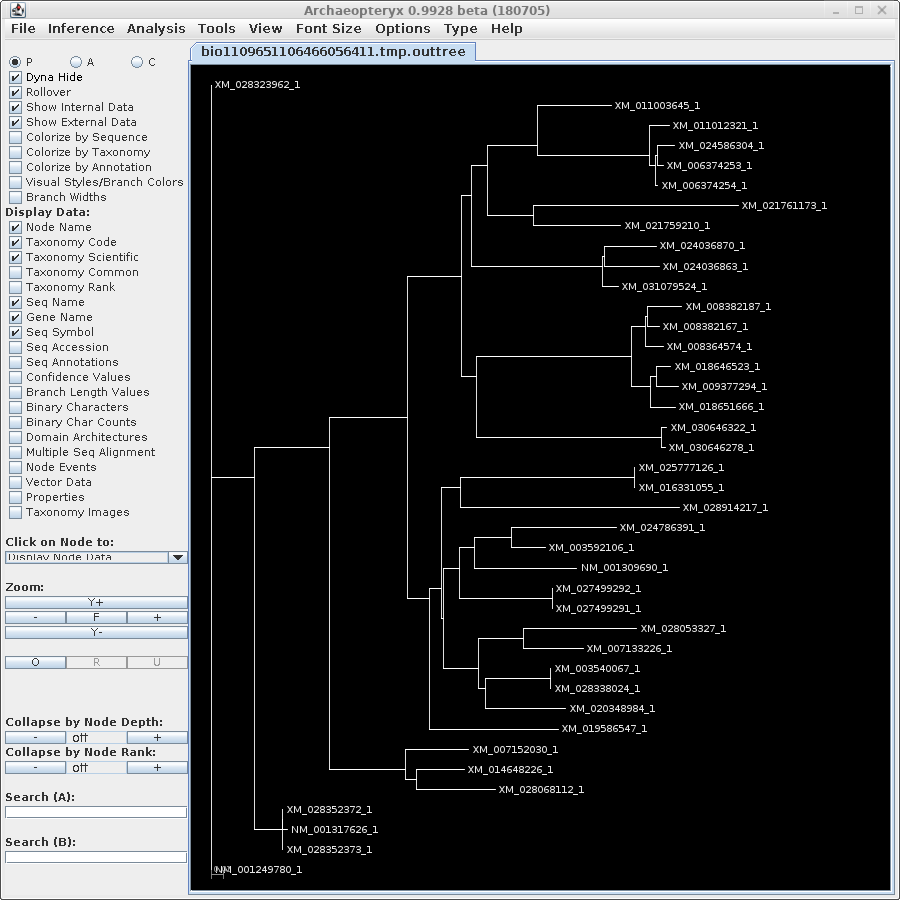
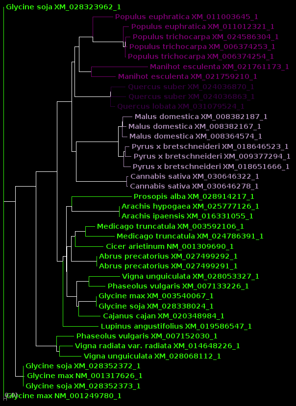
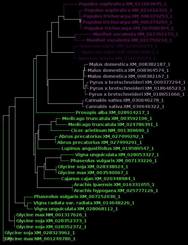
| For now, we will show
results using Archaeopteryx without going into how they were
produced. In a later tutorial, Visualization of Phylogenetic
Trees, we will explore in more depth how to work with
trees in Archaeopteryx. |
| protein |
DNA |
 |
 |