Previous page

TUTORIAL: Genome Assembly de-novo assembly of contigs and scaffolds

December 1, 2023

4. Genome assembly using Abyss

We want to assemble a genome using the three pairs of corrected read files.

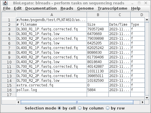Choose File --> guesspairs. As before, we use R1 and R2 to identify paired-end read files, and ask blreads to only select files with the .fq file extension.

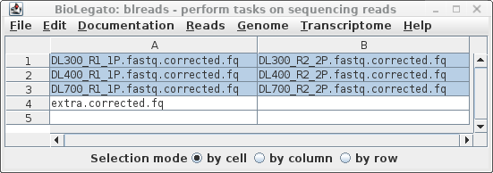
A new blreads window appears with the paired-end files in two columns. Since extra.corrected.fq is empty, we won't bother including that file. Select all pairs of reads, and choose Genome --> ABySS.

It is a good idea to specify a descriptive name for this assembly, in this case R.diobovatum. By default, output will be written to a directory called ../reads.trimmed.corrected.abyss. Again, we want to be more precise, so let's call it ../reads.Trimmomatic.pollux.abyss. Since it takes a long time to do an assembly, it is best to set Notify of completion by email to Yes, and type in your email address.  ABySS has a large number of parameters, not all of which are implemented in blreads. You can set additional abyss parameters, as described in the abyss manual page. If you had additional files with mate-pair reads to be used for scaffolding, those can be added in the mate-pair tab, shown at right.

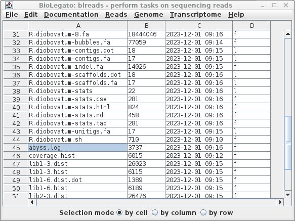
As described in the ABySS documentation, the final genome assembly is found in  R.diobovatum-contigs.fa and R.diobovatum-scaffolds.fa. (These are actually symbolic links to the final contigs in step 6, and the scaffolds in step 8). To see the summary of results, select abyss.log and choose File --> View file.

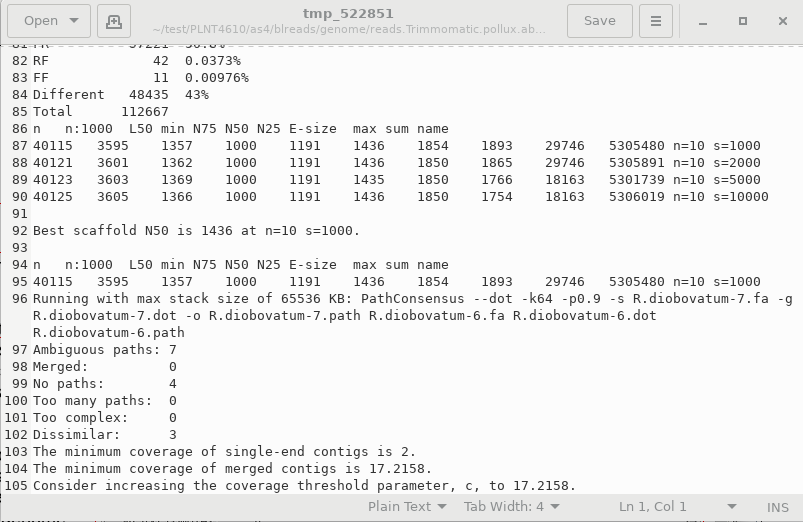
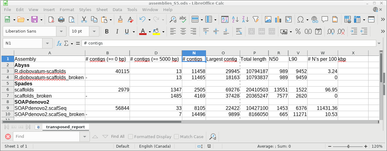
The statistics of the final assembly are shown at the bottom of this file. We see that the number of contigs is 40115, and the median size of scaffold, N50 is 1357 bp. The longest scaffold was 29746 bp. The total size of was about 5.3 million bases. These results would not be good if we were working with a complete set of reads. This test dataset does not have the coverage to give a high quality genome. Since the R. diobovatum genome is over 21 million bases long, less than 1/4 th of the genome is represented in the final scaffolds.

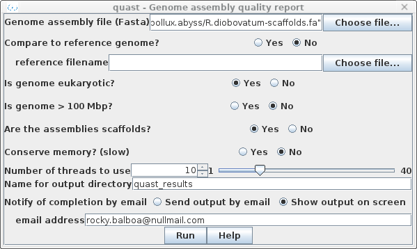
Choose Genome --> Quast. The genome assembly file could either be the contig file, R.diobovatum-contigs.fa, or the scaffolds file, R.diobovatum-scaffolds.fa. The latter us normally preferable. Since this genome is from a fungus, set Is genome eukaryotic to Yes. As well, if the input is scaffolds, set Are the assemblies scaffolds? to yes. Unless your system has very limited memory, it is best to leave Conserve memory to the default setting of "No". By default, output is written to a directory called quast_results.

When quast is complete, files from the quast_results directory will pop up in several windows.


Going clockwise from the top, we see

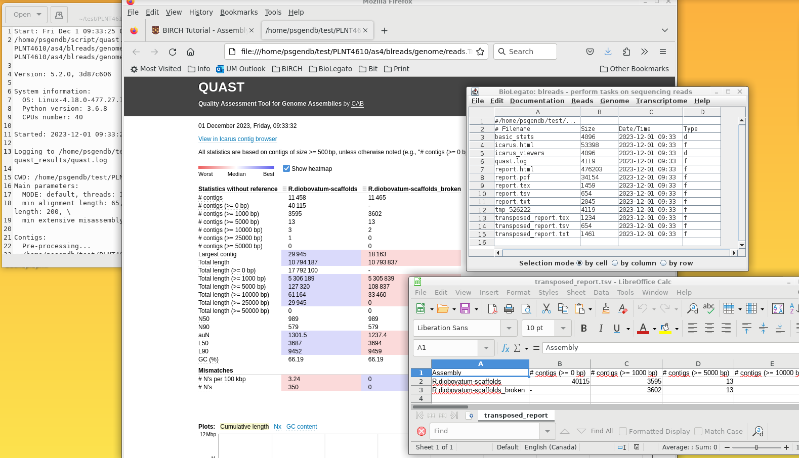
1) quast.log - the details of the quast run
2) report.html - a detailed report of quast statistics, including graphs
3) blreads - showing all files in the quast_results directory. Files can be selected and opened using File --> View file.
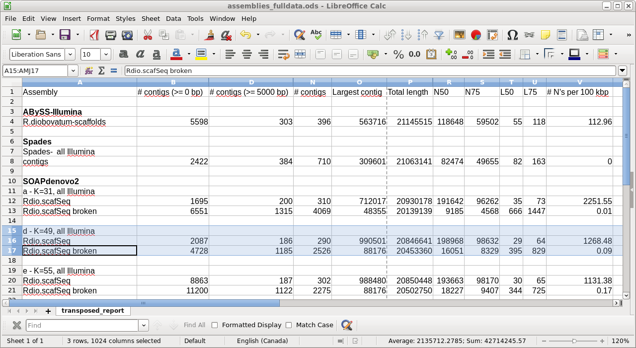
4) transposed_report.tsv - This file contains the same statistics as in report.html, but in spreadsheet form. This is actually a very useful file, because you can copy the lines from this spreadsheet into a master spreadsheet for different genome assemblies, making it easy to compare assemblies for each criterion in the spreadsheet. For example, in the next section, we will assemble the same genome using Spades, and then compare the results from both assemblies in a single spreadsheet.

5. Genome assembly using Spades

Spades has its own read corrector, and spades seem to construct better assemblies when read correction is done by spades, rather than pollux. Start blreads in the reads.Trimmomatic directory, and run guesspairs to select P.fastq files.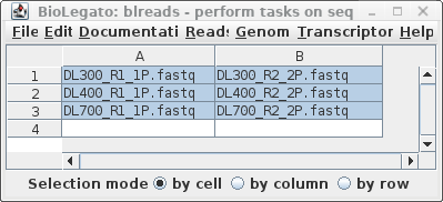

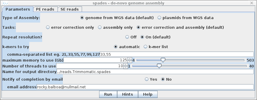
By default, spades will do error correction as the first step. Unless a k-mer list is supplied under k-mers to try, spades will automatically repeat the assembly with k-mers of sizes chosen by spades. To document the steps done, set the name of the output directory to ../reads.Trimmomatic.spades.

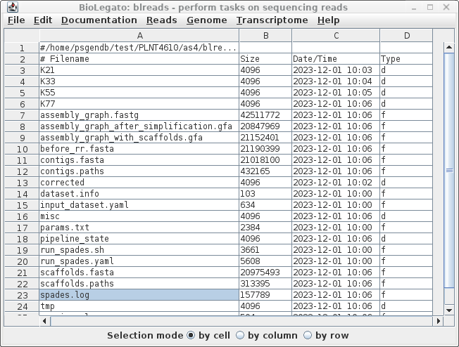
As described in the Spades documentation, spades will try constructing the contigs using several sizes of k-mers (21, 33, 55 and 77). The final contigs will be found in contigs.fasta, and scaffolds in scaffolds.fasta. Where mate pair sequences are not available, there will not be a great deal of difference between these two files.  To see a summary of the results, select spades.log and choose File --> View file.

6. Genome assembly using SOAPdenovo2

• Use reads for contigs and scaffolds, contigs only or scaffolds only
• Average insert size
• reversal of reads in the library (Yes or No)
• rank - order in which libraries are to be used
  
• maximum read length

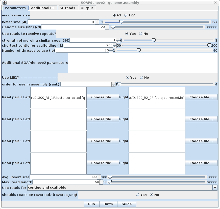
The reads for the first library, as well as global parameters, are set in the Parameters tab. (For longer reads (eg. >250), max. k-mer size would be set to 127.) With this example, the best results were obtained setting k-mer size to 31, which is about 1/5 the size of the sequencing reads. The expected genome size is 21 Mb, so set Genome size to 24 Mb to make sure enough RAM is used. For eukaryotic genomes, it is always best to set "Use reads to resolve repeats" to Yes. In this example, the first library, LIB1, has left and right members chosen for Read Pair 1, with Avg. insert size set to 300 bp inserts. The Max. read length for these reads has been set to 150 nt.

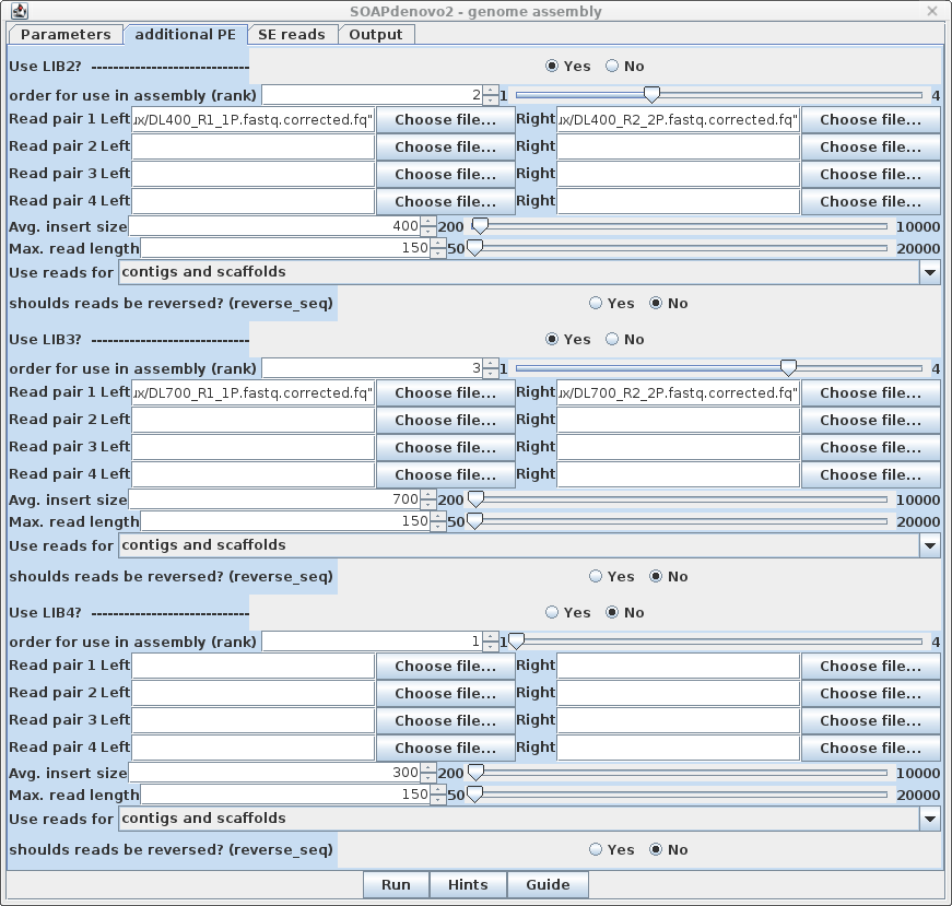
This assembly also has files with 400 and 700 bp inserts, so we specify these files and their parameters in the AdditionalLIBS tab. For the 400 bp inserts, click Yes for Use LIB2 and set rank to 2. Set Avg. insert size to 400, and Max. read length to 150. Similarly, for the 700 bp inserts, click Yes for Use LIB3 and set rank to 3.  Set Avg. insert size to 700 and Max. read length to 150. Note on mate pair reads: If you are using mate pair reads for scaffolding, put these in a separate library and set Use reads for scaffolds only.

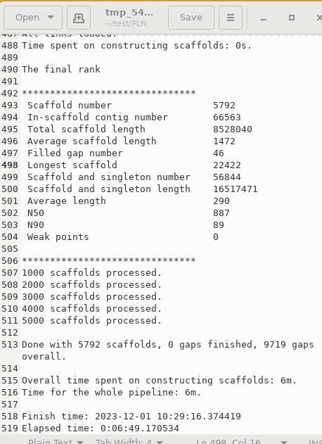
An example of output as shown in soapdenovo2.log, is shown at right.

7. Comparison of assembly statistics

To make the results easier to compare, title lines for Abyss, Spades and SOAPdenovo2 have been added. As well, some columns have been hidden to make it easier to see a number of important columns at once.

In summary,

• Spades gives us fewest contigs than Abyss and SOAPdenovo2 and the N50 is larger for Spades (13551) than for Abyss (989) or SOAPdenovo2 (1453).
• Spades has far more contigs of large size (1347) versus Abyss (13) or SOAPdenovo2 (33)
  
• Spades also has the largest contig (69276) versus Abyss (29945) or SOAPdenovo2 (22422)
  

By these criteria, the Spades assembly for these reads is much better than the other assemblies.

What about the full dataset?

It is critical to remember that the results from this sample data are not representative of what you would expect if a much larger set of reads had been used. The sample dataset does not have anywhere near the coverage needed for a good genome assembly. We have used a small subset of the reads to give you an idea of the process of genome assembly,  so that assembling a genome for a complete set of reads should be straightforward.

Below is a comparison of assemblies using the same three programs with the full dataset.


assemblies_fulldata.ods

With full coverage, SOAPdenovo2 gave far better results than ABySS or Spades. Three different k-mer values are shown for SOAPdenovo2, which illustrates that an optimal choice of k-mer can have have a major influence on the quality of the assembly. Too small a k-mer value and the program will fail to consider many potentially good paths in the de Bruijn graph, resulting in shorter contigs. Too large a k-value (ie. too close to the read size) will have the effect of artificially decreasing the coverage for some contigs, again preventing contig extension, and/or resulting in incorrect scaffolding.