
Why do we still need genetic mapping? Can't we just sequence the genome?
No matter how sophisticated and rapid DNA sequencing and other genomics technologies become, there is still no getting around the fact that what we're really interested in, in practical terms, is phenotypes. We want to somehow get at traits that are responsible for diseases in humans, or for agronomically useful characteristcs in crop plants and livestock. Examples of the latter would include disease resistance, yield, protein quality, oil quality, or uniform height or flowering time. Many of these traits are quantitative traits, governed by multiple loci. In many cases, the only thing we know at the beginning is the phenotype. Consequently, Mendelian genetics is more relevant than ever, as the primary way to go from a trait we can see or measure, to a specific chromosomal locus and gene product.
Mapping genes to chromosomal loci used to be done using 3 point crosses. Now, the process is almost completely based on molecular markers. Using molecular markers provides many advantages, including:
But also -
Modern genetic mapping using molecular markers still relies upon the basic principles of Mendelian genetics. We observe genetic segregation based on the segregation of alleles in genetic crosses. But for molecular markers, we need a broader molecular definition of what an allele is. The word "allele" comes from the earlier word "allelomorph", which simply means "other form". We can use allele to mean a different trait, in a phenotypic sense, or to mean a different sequence, in a molecular sense. An allele defined by molecular means should have exactly the same genetic properties as a phenotypically-defined allele.
Infinite alleles model : Mutations within protein
coding sequences define molecular allelism at many levels
and degrees of severity.
Mutations can take many different forms. Some mutations may have more of an effect than others:
| Mutation Type | Translaton |
Effects |
|---|---|---|
| No mutation | GAU CGA UGC CAG Asp-Arg-Cys-Gln |
This produces the wild-type protein |
| Silent mutation | GAU CGA UGU CAG Asp-Arg-Cys-Gln |
Although one base pair has changed from C to U, both codons still produce a cysteine, and the end product is unchanged. No effect on the protein. |
| Missense mutation | GAA CGA UGC CAG Glu-Arg-Cys-Gln |
This mutation, changing a U to an A, changes the sequence of amino acids. A missense mutation can have varied effects depending on how similar the mutated amino acid is to the original. In this case, Glu and Asp are similar, so the effect may be low. |
| Nonsense mutation | GAU CGA UGA CAG Asp-Arg |
A nonsense mutation results in the early termination of an amino acid sequence. Instead of getting UGC, for cysteine, we get UGA, a stop codon. This type of mutation can range from very severe, if it occurs early on in the sequence, to less severe when it occurs closer to the end. |
| Frameshift mutation | GAU GAU GCC AG Asp-Asp-Ala |
A frameshift mutation results from either an insertion or deletion, and is named because it shifts the frame of reference. As you can see, that results in a completely different amino acid sequence. Sequences that suffer frameshift mutations are often heavily effected, and are likely non-functional. |
In addition to these point mutations, there
are also large-scale sequence changes as the result of large
insertions or deletions, as well as rearrangements. Not all
mutations are necessarily bad - since the eukaryotic genome
contains lots of "junk" DNA, often mutations do not affect
organism functioning at all. If mutations occur on a non-essential
portion of a large protein, the difference might be very small.
| Divergence of protein sequences during plant evolution. Amino acids from the N-terminal region of thionin proteins from several plant species are shown. Where amino acids have been inserted or deleted during the course of evolution, gap (-) characters have been inserted to optimize the alignment of homologous positions within the proteins. | |
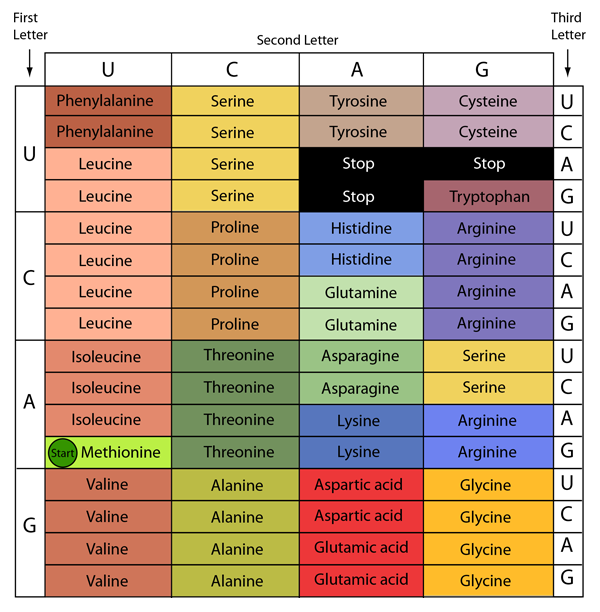
Of course, part of the reason that sometimes mutations don't have a big effect on function is the degeneracy of the genetic code. By "degenerate", we mean multiple codons can code for the same amino acid:
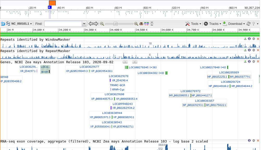
Since only a small percentage of eukaryotic genomes codes for proteins, most mutations will occur within non-coding DNA, and will usualy be selectively neutral. In most eukaryotic genomes, the chromosome is a sea of non-coding DNA punctuated by genes. This is illustrated in an approximately 1 Mb region taken from Zea mays chromosome 6:
Additionally, genes are composed of both exons and introns. In comparison to exons, introns appear to mutate very rapidly, suggesting that there is little selective pressure against intronic mutations. In many higher eukaryotes, especially in animals, introns may be very long compared to exons (Note that this appears not to be the case in plants, in which introns tend to be short).
In conclusion:
Practical consequence: because most mutations are selectively neutral and can occur anywhere in the genome, we can use molecular alleles as markers for chromosome mapping.
At this point, we've discussed restriction digests, and you're familiar with the idea that when we digest a sequence with a certain restriction enzyme, we get bands of different lengths. Now, what happens when that particular sequence has differences between alleles? Well, we see polymorphism in the fragment lengths. Restriction sites can be assayed for polymorphism within a population by Southern hybridization - and these restriction sites can reveal polymorphism between genomes.
 Assuming that individuals 1
and 2 are homozygous at the locus detected by these probes:
Assuming that individuals 1
and 2 are homozygous at the locus detected by these probes: 
DNA sequences are mutating all the time. As two populations
diverge over time, they each accumulate different mutations at
different sites. When restriction sites in the vicinity of a given
gene are compared from one genotype to another, one genotype may
have the site, and the other will not. This is referred to as a
polymorphism. High polymorphism between two genotypes is evidence
of genetic divergence. Mike Freeling and colleagues have compared
restriction sites within the maize alcohol dehydrogenase 1 (Adh1)
gene in several maize lines. They found that although the
restriction maps are identical within the Adh1 gene for all
varieties tested, very few of the restriction sites outside of the
coding region are conserved.
Johns, M. A.,
Strommer, J.N. and Freeling, M. (1983) Exceptionally high
levels of restriction site polymorphism in DNA near the maize
Adh1 gene. Genetics 105:733-743.
| Maize
genomic DNA was digested usng HindIII and the bands analyzed
by Southern blot hybridization. DNA from seven maize lines
was compared. The blot was hybridized using the pZmL84
probe, whose location on with respect to the AdhI gene is
shown in the figure below. Note that this probe overlaps the
3' half of the adh1 transcript. Since the HindIII site is internal to the probe region, the probe detects two bands in all digests. In all maize lines, a conserved 2.5 kb fragment is seen, as well as a second band. The size of the second band is determined by how far away the next HindIII site is, downstream from the conserved HindIII site. Because numerous mutations have accumulated in the downstream region, in the different maize lines over time, the location of the downstream HindIII site differs between lines. |
 |
A restriction map of the corresponding region of the adh1
locus is shown below.
| Restriction maps of the seven Adh 1
chromosomal regions. The boundaries of the transcription
units are denoted by the vertical dashed lines, and the
region that hybridized with the ADH1-cDNA probe, pZML84, is
also shown. In all lines the 5' fragment detected by the pZmL84 probe is 2.5kb. The map shows that the two HindIII sites that define this fragment are conserved. The 3' fragment is different in each line, because the next distal HindIII site occurrs at a different location in each line. |
 |
Now that millions of genes have been sequenced from thousands of
species, we can generalize that protein coding regions are
typically slow to diverge, because there is usually selective
pressure to retain a given amino acid sequence. Outside of the
protein coding region, and in non-coding DNA flanking genes, there
is little selection against random mutations. Hence mutations are
allowed to accumulate quickly in non-coding regions.
Each band seen in a Southern blot indicates the presence of one or more restriction sites in a sequence. The sequence containing a restriction site is one allele, while the corresponding sequence missing the restriction site is the other allele. The "phenotypes" of these alleles are the differences in banding patterns, due to presence or absence of bands. In most cases, both loci have bands from one parent or or the other, or both loci are heterozygous. These are parental genotypes. When one locus is heterozygous and the other is homozygous, they must be recombinant. It is important to note that the %recombinants in F2 analysis doesn't give you the recombination frequency. Consider the case in which two recombinant gametes join to form a zygote:

These progeny would be heterozygous at both loci, which might be naively scored as non-recombinant. This is why geneticists have traditionally gone to great extremes to construct tester-stocks for mapping by test crosses. However, that is not always possible to do, especially if you want to map hundreds or thousands of markers to construct a genomic map. Consequently, you have use analytical methods appropriate for F2 data.
In a two point test cross, calculating linkage between two loci follows this formula:
When we look at the last example, it's clear that we are not able to get accurate linkage values from a two point test cross. Where we're looking for homozygotes, we miss the recombinant progeny that are heterozygotes, and end up with an inaccurate linkage for those two loci.
However, once we are dealing with multiple
markers, it gets much more complicated. To get an idea about how
molecular marker data can be used to build linkage maps, let's
examine some molecular markers from TAIR (The Arabidopsis
Information Resource) at Stanford University. One of the RFLP
probes documented in AAtDB is the RFLP probe g4539, which can be
examined here. (Note: In the current map,
g4539 has been converted into a PCR marker.) The Southern blot
for this probe, shown at right, indicates two RFLP alleles, 2L
and 1C, found in ecotypes Landsberg erecta and Columbia,
respectively. Note that while several bands are detected with
this probe, only two are polymorphic between these two parents:
2L and 1C.
If you take marker g4539 as an example, you will see that
neighboring markers most closely-linked to it also are most
alike in the phenotypic scores, from plant to plant. The farther
you go in either direction from g4539, the more different will
be the scores. Neighboring loci in any region will always have
the most similar segregation patterns. This is nothing new, it
is simply a restatement of the idea of co-segregation of
closely-linked loci. By definition, the more closely-linked two
loci are, the more they will cosegregate.
------------- segregating progeny -------------------> marker/ |
When we calculate linkages for multiple loci at once, we use maximum likelihood methods. These methods follow two simple steps:
In Fig. 1, we see that MAPMAKER begins considering a particular map in the following way:
As the iterations progress, the changes to the map get smaller and smaller. The process repeats until the difference in log likelihood between the current map and the previous map is less than some threshold (eg. 0.1). In this way, the program quickly converges on the spacing that is most consistent with the data.