Doggett, NA. et al. (1995) An integrated physical map of human chromosome 16. Nature 377:335-365.
The following table gives both physical map lengths of each human
chromosome, as well as total genetic length, based on genetic
recombination.
| |
Physical map (Mb) | Genetic map (cM) | Number of markers | ||
| Male | Female | Sex Average | |||
| 1 | 282 | 195 | 345 | 270 | 468 |
| 2 | 252 | 190 | 325 |
257 |
407 |
| 3 |
225 |
161 |
276 |
218 |
369 |
| 4 |
205 |
147 |
259 |
203 |
302 |
| 5 |
199 |
151 |
260 |
206 |
334 |
| 6 |
191 |
138 |
242 |
190 |
293 |
| 7 |
169 |
128 |
230 |
179 |
246 |
| 8 |
158 |
108 |
210 |
159 |
247 |
| 9 |
150 |
117 |
198 |
158 |
193 |
| 10 |
146 |
134 |
218 |
176 |
256 |
| 11 |
153 |
109 |
196 |
152 |
260 |
| 12 |
153 |
136 |
207 |
171 |
239 |
| 13 |
100 |
101 |
156 |
129 |
175 |
| 14 |
87 |
94 |
142 |
118 |
161 |
| 15 |
87 |
103 |
155 |
129 |
125 |
| 16 |
106 |
108 |
150 |
129 |
151 |
| 17 |
89 |
109 |
162 |
135 |
181 |
| 18 |
89 |
99 |
143 |
121 |
158 |
| 19 |
69 |
93 |
127 |
110 |
120 |
| 20 |
59 |
75 |
122 |
98 |
141 |
| 21 |
30 |
47 |
76 |
62 |
67 |
| 22 |
31 |
49 |
83 |
66 |
67 |
| X |
156 |
- |
179 |
179 |
66 |
| TOTAL | 3191 | 2591 | 4460 | 3615 | 5136 |
| Kong A et al. (2002) A high-resolution recombination map of the human genome. Nature Genetics 31: 241-247. | |||||
Total genome size: 3191 Mb
Male
linkage
(total): 2591 cM
Female
linkage
(total): 4460 cM
Sex
average:
3615 cM
3191
Mb
÷ 3615 cM = 883 kb/cM
As these data show, the average physical length of 1 cM in the human genome is 883 kb. The actual physical distance that 1 cM corresponds to will change depending on the organism under study. This has something to do with the frequency of recombination.
Think of it like this: if an organism has more frequent recombination overall, the map distances based on recombination will increase. After all, the higher the chance of recombination the larger the relative distance. However, the physical distance will not change. Let's look at Arabidopsis thaliana as an example.
The A. thaliana genome is 7 x 10⁴ kb long,
physically (Nam et al. (1990) Plant Cell 1: 699-705). It has a
total length in cM of 437. Therefore, each cM represents 160kb of
DNA. This is a much lower number than the one for the human genome
above, indicating that it has a higher amount of recombination. So
why does Arabidopsis have more frequent
recombination?
Does it have something to do with the fact that it has very little
repetitive DNA? Wouldn't that decrease recombination frequencies?
Genetic distances, measured by recombination, are not always linearly related to actual physical distance. When we calculate recombination frequency, we use a unit of distance called a centi-Morgan (cM). A genetic distance of 1 cM represents a 1% chance that the loci in question will be separated due to recombination in one generation. In this way, centiMorgans represent relative distance between markers. Absolute distance, or physical distance, is measured in the familiar unit of base-pairs (bp, kbp, or Mbp/Mb).
| For example, a comparison of physical and
genetic distances on human chromosome 16 shows that the
physical distance corresponding to 1 cM (map unit) varies
along the length of chromosome 16. The markers D165S309 and
D16S83 are practically next to each other on the chromosome,
but have a very high frequency of recombination between
them. Additionally, the markers SPN and D16S300 have ~25Mb
between them, and almost no recombination. Doggett, NA. et al. (1995) An integrated physical map of human chromosome 16. Nature 377:335-365. |
|
So far, we've only been talking about one kind of molecular marker: RFLPs. In principle, any method that can identify mutations at any chromosomal location can be used to mark a site on a chromosome. RFLPs can be time consuming and expensive, so it's not always feasible to use them. PCR-based methods offer an alternative to RFLPs, and can be used for all the same purposes as RFLPs.
Since variation in repeat number gives PCR bands of different sizes, each band represents an alleleMicrosatellites, also called variable number of tandem repeats (VNTRs) lend themselves to length polymorphisms, most likely because of strand slippage during DNA replication. The net result is that it is easy to find polymorphic microsatellites in which different alleles have different numbers of repeat units, so that the total length of a given microsatellite locus may vary. In other words, each variant is a unique allele at that locus. For a given locus containing a microsatellite, PCR primers specific for that locus are designed from the unique sequences flanking the repeats. Thus, microsatellite alleles are usually based on length polymorphism. Polymorphism at the priming sites would result in loss of bands, rather than changes in length. |
 |
For a given locus containing a microsatellite, PCR primers specific for that locus are designed from the unique sequences flanking the repeats. Thus, microsatellite alleles are usually based on length polymorphism. Polymorphism at the priming sites would result in loss of bands, rather than changes in length.
Example (link provided for background reading): Aarnes SG et al. (2015) Identification and evaluation of 21 novel microsatellite markers from the automnal moth (Epirrita autumnata) (Lepidoptera: Geometridae). Int. J. Mol. Sciences 16:2241-22554. doi: 10.3390/ijms160922541.
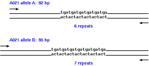
| The authors identify a number of microsatellite loci in the autumnal moth, which are polymorphic for the number of copies of short tandem repeats. Both alleles for each microsatellite locus were sequenced to determine the number of copies of tandem repeats in each, and the total length of the bands generated. For example, at locus A021 allele A contains 6 repeats of TGA, resulting in a PCR band whose total length is 92 bp, while allele B contain 7 copies of the TGA repeats, giving a PCR band of 95 bp. |
 |
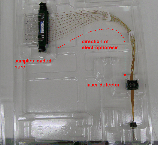
| Typically, several microsatellite loci can be amplified in a single PCR reaction. For each locus, primers for each locus are tagged with distinct flourescent dyes, so that the microsatellite bands for each locus flouresce at different wavelengths. PCR fragments are generated in separate reactions for each locus each using a different dye. After amplification, samples are mixed, and separated by capillary electrophoresis. This technique, rather than using a slab gel, runs DNA fragments through a thin capillary tube, containing polyacrylamide gel. A laser detector at the end of the capillaries detects the signals for each band at their characteristic wavelengths. |
 |
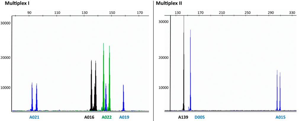
Results appear in a chromatogram, in which each DNA band appears as a peak. Bands for both alleles at each wavelength would fluoresce at the same wavelength. Homozygous loci, in which only one allele are present, give a single band eg. loci A019, A139 D005. Heterozygous loci, in which both alleles are present, give two bands eg. A021, A016, A022, A015.
There are many different schemes for detecting polymorphism (ie. differences in a given sequence among members of the population). Any of these can be used for molecular markers.
Regardless of the type of molecular marker employed, each assays a single genetic locus. That is, each marker assays a region of d cM on both sides of the marker. Another way to conceptualize it is to say that the genome is divided into G/2d segments of 2d each.
What you might be tempted to do is to say that the numbers of markers to score, to cover the entire genome, is the genetic distance of all chromosomes added together (G), divided by the genetic distance covered by each marker.
N = G/d
Where N is the number of markers necessary to have at least one
marker within d map units of any gene.
Note: As calculated here, N is referred to as "1 genome
equivalent".
The problem: N randomly chosen markers will be scattered unevenly across the chromosomes, so some regions will be full of markers, and other regions will not have any markers at all.
| What we have to do, then, is to saturate the genome with markers, to ensure every region is covered. An initial map might be constructed using a relatively small number of markers. Since the chosen represent a random sampling of loci, they will be distributed unevenly across the genome. Consequently, some regions of each chromosome will be overrepresented in the map, and others will be underrepresented. As we sample more markers and add them to the map, their map locations will also be unevenly distributed. Finally, if enough markers are used, there will always be at least one marker with in a certain distance d of any part of the genome. |
 |
Therefore, it is necessary to screen a large number of markers
before you find one that is linked to your gene. The following
equation [Clark and Carbon (1976) Cell 9:91] allows us to
calculate the number of markers necessary to find one that is
linked to the gene of interest:
where:
| For example, to find a marker in the human genome (3615 cM) linked within 10 cM of any gene, |
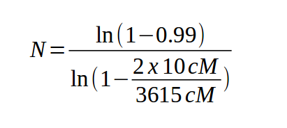 |
Now, the bad news here is that 830 is a lot of markers, and will be expensive. But the good news is that we've set the value of P high, to make sure we do find a marker linked to the gene of interest. However, if we set P equal to 0.5 (50%) we only have to look at 124 markers. We can rephrase this as "50% of the time we only have to look at 124 markers before finding a marker linked to the gene". If we set P equal to .75, the number of markers becomes 250. So, just because 830 is our result doesn't mean that the marker linked to the gene will be the 830th marker every time. Rather, it means that to be 99% sure we're getting a marker linked to our gene we have to look at 830 markers.
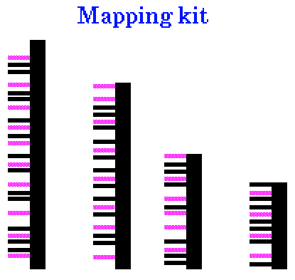
The examples above show that if you are trying to find a marker linked to a gene of interest, just screening randomly-chosen markers requires that a large number of markers be screened to be sure that at least one is linked to your gene. However, once a genome has been saturated with markers, you only need to search a small set of evenly spaced markers that together cover the entire genome. That way, no matter where your gene is, at least one of the markers you screen must be closely-linked with your gene. A mapping kit is a set of markers that are evenly spaced on the chromosomes. If you can define a minimal set of markers, you can detect linkage by testing a minimal number of probes. One way of looking at it is that now that we have saturated the genome, we can choose a set of evenly-spaced markers so that N = G/2d. For example, if the human genome is 3615 cM in length, and we have markers evenly spaced at 20cM distance, then we need only 3615/20 = 181 markers to detect any gene.