Let's start by giving an example of what it is most genome programs hope to accomplish. Conceptually, this can be broken down into successive steps, each at a finer level of resolution:
The result in an integrated model of the genome. The first genome to be entirely mapped was that of the nematode worm, C. elegans. The original 1998 sequence has since been updated to correct small gaps. The NCBI homepage for C. elegans can be found here. Some of the genome data from NCBI is presented below:

Ideally, all genome mapping projects would be able to produce a result of this quality.
A library is a random set of clones, in which genomic sequences
are represented (in the ideal) by a Poisson distribution within the library. In
other words, because cloning is a largely random process, some
sequences will be cloned several times, and others with be cloned
very rarely. Consequently, it is necessary to use the Clark &
Carbon formula to determine how many clones are necessary to be
sure, within a certain probability, of encountering each sequence
at least once. Some sequences which are hard to clone may be
statistically underrepresented in the library.
| A genomic library is a
population of clones, each containing a unique fragment of
genomic DNA, which together, represent the entire genome. As illustrated at right, if you have only a few clones, they are likely to be from different parts of the genome. As you keep drawing clones from the library, more and more sites in the genome are represented. Because clones are chosen at random, some parts of the genome will be overrepresented, while for other parts of the genome, no clones will have been chosen (second stage). Finally, if you choose a large enough number of clones, you can be sure that every part of every chromosome is represented in at least one of the clones (third stage). The Clarke and Carbon equation from last reading allows us to calculate the number of genomic clones necessary to construct a genomic library:
Where:
|
 |
As an example, let's use the BAC average insert size (0.1 Mb) and the Arabidopsis thaliana genome (70Mb).
f = 0.1Mb / 70Mb = 1.43 x 10⁻³
N = ln(1-0.99)/ln(1-1.43 x 10-3) = 3218
Note: make sure you adjust the units so that they match!
Just to put things into perspective, you could call 1/f one genome equivalent, that is, if you could split the genome up into adjacent segments of 100 kb, you would need 1/f segments to represent each piece of the genome once. This would be 700 clones for Arabidopsis. But, we have shown that to have a 99% chance of getting a given gene, you need to screen 3218 clones, so:
3218/700 = 4.6 genome equivalents
| Organism name | Genome size (Mb) | Insert size (Mb) | Genome equivalents needed (with BAC) | ||
|---|---|---|---|---|---|
| Lambda (.02) |
Cosmid (.035) |
BAC (.3) |
|||
| E. coli | 4.5 | 1034 | 590 | 67 | 4.47 |
| A. thaliana | 70 | 1.6 x 10⁴ | 9208 | 107 | 4.59 |
| H. sapiens | 3000 | 6.9 x 10⁵ | 3.9 x 10⁵ | 4.6 x 10⁴ | 4.6 |
| P. sativum | 4600 | 1.1 x 10⁶ | 6.1 x 10⁵ | 7.1 x 10⁴ | 4.63 |
| The insert size of 0.3 Mb for BACs is an optimistic figure, although some libraries have inserts this large. | |||||
This table indicates that on average, around 4.5 genome equivalents are need to have a 99% probability of getting every sequence at least once.
The bigger the insert, the fewer clones you need to span a given region. In principle, there is no upper limit to the size of inserts YACs can hold. Furthermore, YACs can replicate as a plasmid in E.coli and as a chromosome in yeast. So why not clone in YACs? Well, YAC vectors have been created, and while the size of inserts is virtually unlimited, there are several critical problems with YACs:
The term "BAC" stands for Bacterial Artificial Chromosome, but it important to remember that these are prokaryotic artificial chromosomes, that is they are designed to replicate in bacteria, not in eukaryotic cells. While BACs are actually derived from the E. coli F' plasmid, BACs are distinct from ordinary plasmids by having a number of features to optimize the ability to work with large inserts.
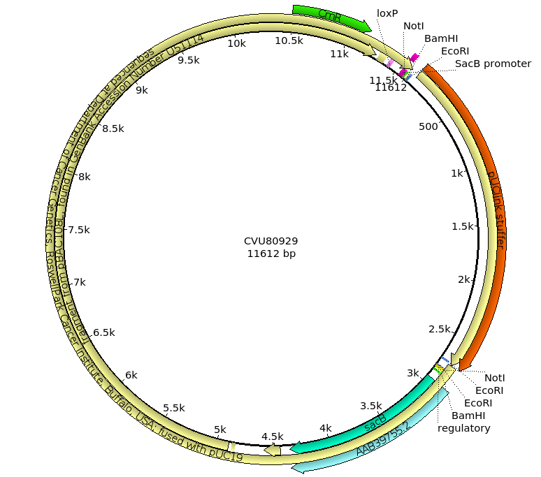
In the figure above, the multiple cloning sites that we would expect to see in a vector are present, as well as an ori site. However, there are some slight differences from the vector we've seen before:
When we are working with large inserts, it's more efficient to use restriction enzymes that have longer recognition sequences, because they cut less frequently and therefore create longer insert fragments. For example, the NotI enzyme has an 8bp recognition sequence, while BamHI and EcoRI have 6bp recognition sequences. On average, using NotI instead of BamHI or EcoRI will result in fragments that are an order of magnitude larger.
While BACs have a number of advantages, namely:
...there are also some disadvantages. While 350 kb fragment sizes is an improvement, there would still need to be many, many clones made to cover large genomes, in particular. Additionally, there are some sequences that are hard to clone in E. coli, and therefore may also be missed in BAC libraries.
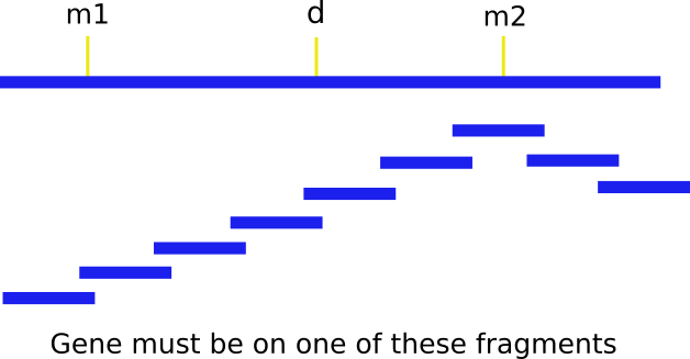
Given a molecular marker, how can you clone the associated gene? The first step in this process is to localize to a small area using genetic crosses. Map the gene you want to clone (d in the figure below) to a position between two markers (m1 and m2).

Keep in mind, though, that a map distance of even 1 cM can correspond to a large kilobase range! In A. thaliana, 1 cM is equal to 160kb, while in humans, 1 cM is equal to 883 kb! Although this may seem like a small distance to examine, it's larger than it looks - and there could be a lot of genes in one map unit.
The next step is to assemble a contig by chromosome walking. Starting from one of the markers (let's use m2), you "walk" along overlapping fragments until you find the gene. It's important to note that during the initial walk, you have to walk in both directions, since you don't know whether the gene is upstream or downstream from m2. Generally, you can determine directionality two ways: by simply walking in both directions until you find m1, or if one of the overlapping clones detects a polymorphism. This facilitates a 3 point cross with the probe, m2 and d.
How do we find these fragments that overlap so nicely? These fragments, or probes, are called end-specific because only the ends overlap with the next probe, making it so we can assemble contigs easily while covering the most area. Here's how these end-specific probes are made:
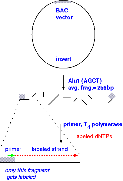
If you user a primer synthesized to match the region of the vector immediately flanking the insert, the labeling reaction will proceeed into the insert, and terminate at the end of the fragment, where AluI cut. One of the advantages of this approach is that the same primer can be used for all clones, because all inserts are in the same vector!
End-specific probes can be used to assemble a contig - a set of overlapping BAC clones. Each time an end-specific probe identifies a new clone in the library, one step in genome walking has been taken.

From this point on, every gene is a special case. You know that the gene you're interested in is on one of the clones, but which one?
Complementation is the method of choice for experimental systems that allow transformation. For example, disease resistance genes in plants have been cloned by transforming susceptible plants with DNA from each BAC in a contig, and screening for resistant plants.
cDNA screening is an approach that sometimes works. eg. screening for a disease gene in humans:
An ordered library is a library of overlapping clones, such that each sequence outside of overlap regions is represented exactly once. Put another way, think of the chromosome as being split into short fragments laid end to end. Contigs are assembled by successive hybridization, fingerprinting, or sequencing experiments. Since thousands of clones have to be compared against each other to detect overlaps, computers are used to do pairwise comparisons. |
 |
In the past, genomes were sequenced by first making a BAC library, and then sequencing enough clones to cover the entire genome. Even today, these genomes are among the best genomic sequences. However, the time and expense of this strategy makes it impractical for sequencing large numbers of genomes. Whole genome shotgun sequencing is a quicker and cheaper way to sequence genomes, but has the disadvantage that most of the time, full chromosomal sequences cannot be built for eukaryotic genomes. The trade off, then, is between cost and speed, and completeness of the genomic sequence.
Further reading: Ekblom R, Wolf JBW (2014) A field guide to
whole-genome sequencing, assembly and annotation. Evolutionary
Applications 7: 1026 - 1042. Link
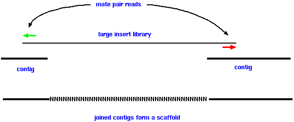
| An overview of whole genome shotgun sequencing. A mate-pair read is sequence information from two ends of a DNA fragment, usually several thousand base-pairs long. A scaffold is two or more contigs joined together using read-pair information. Within a scaffold, the gaps between adjacent contigs are usually denoted by a run of N's. | 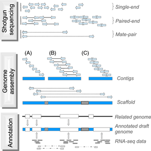 |
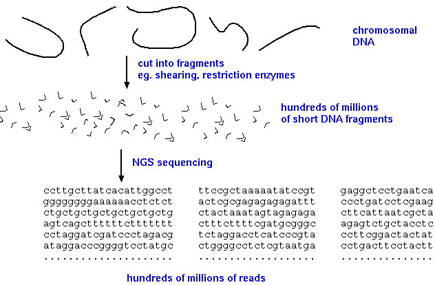
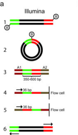
WGS begins by creating a library of fragments from genomic DNA. Usually a PCR step amplifies the fragments, which are a uniform size, depending on the specific sequencing technology used. For example, with Illumina technology, fragments are typically about 300 bp in length. Since sequencing reads can be 150 bp or longer, it is possible to get two paired-end reads that overlap, to cover the entire 300 bp fragment. |
 |
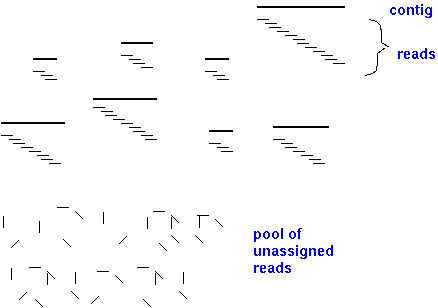
Typically, WGS sequences enough reads to cover the entire genome with 50 to 100-fold redundancy. Highly-efficient pattern matching software pieces together reads at points of overlap to form contigs. The algorithm keeps adding reads together until contigs can no longer be extended from the pool of reads. Generally the bigger the contigs, the better the sequence assembly.
Each contig is assembled from many overlapping reads. At this point, we have no idea which chromosome each contig comes from, or where the contigs might be placed on those chromosomes. There is usually a large number of unmatched reads that cannot be assembled into contigs, and very small contigs (eg. a few hundred or a few thousand base pairs in length) that do not contribute anything to the final genome assembly.
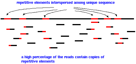
Eukaryotic genomes are especially difficult to assemble because so much of the genome consists of repetitive elements, such as the AluI family, interspersed among unique DNA. Since the length of sequencing reads is fairly short, a high percentage of reads will have part of a repetitive element at one end. Few reads will completely span a repetitive element, with unique sequence on either side. While it is true that repetitive sequence elements do mutate, it is often difficult or impossible for sequence assembly software to decide which copy of a repetitive element to join with any of thousands of other copies that may be identical or nearly identical to the a given read. Put another way, we don't know where on the chromosome each read came from. That is what we're trying to figure out. The net result is that as a growing contig encounters a repetitive element, there may be no way to extend the contig further. Consequently, most genome assemblies have a relatively small number of large contigs, and a very large number of small contigs, maybe 1000 bp or smaller.
With current sequencing technologies, the best strategy for joining contigs is to do a second sequencing run, this time using libraries with large fragment sizes (eg. 3000 bp or greater). The reads from these larger insert libraries are called "mate pair" reads. If we find one read within one contig, and the read from the other mate pair somewhere within another contig, we know that the two contigs are no farther away than the length of the large insert.
Then, contigs can be joined together and assembled into much longer scaffolds. Ideally, we can join many different contigs together to make the scaffold as long as possible.

Scaffolds join contigs in the order and orientation with which they appear on the chromosome. If we're lucky, may be able to assemble scaffolds that completely cover an entire chromosome. Most of the time, though, there are 2 or more scaffolds per chromosome, and we don't know the order and orientation of the scaffolds, relative to one another.
Like all strategies, whole genome sequencing comes with some disadvantages. For most chromosomes, there will be more than one scaffold per chromosome. This means that the overall assembly will have large gaps between contigs, likely missing some genes and large portions of repetitive DNA. In turn, we will likely underestimate the amount of repetitive DNA in the genome. For diploids, the reference chromosome resulting from the assembly is a composite of both copies of a chromosome pair.
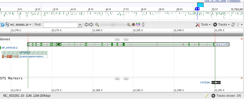
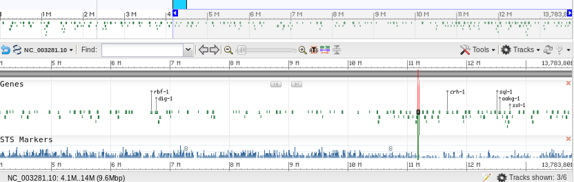
If you want to look at genome sequences that have been assembled, you can view them here. Note that often there are some scaffolds without a determined location.
After building a full genetic map, we have the DNA sequence, gene locations, and a sense of the overall arrangement of the chromosomes. One of the other pieces of information that we can add to the genetic map is how much and how often genes are expressed. This information is partially contained in the transcriptome: the the set of all RNA transcripts expressed in an organism. High throughput RNA sequencing can be used to measure the amount of each of thousands of distinct RNA transcripts in an RNA population.
Gene expression studies tend to generate two different types of data. Studies in which two or more conditions are compared at a time generate discrete state data. Often it is critical to follow the expression of a gene over time after a treatment. In timecourse experiments, the expression of each gene in response to two or more treatments is measured over time. For example, in the timecourse at right, the solid blue and red dashed curves might represent the expression levels for a gene in response to two different drugs.
| What we're ultimately trying to get from gene expression experiments is expression patterns for each of the thousands of transcripts in the RNA population. By identifying genes whose expression patterns are similar, we can discover which groups of genes work in concert, in response to a given stimulus. |  |
There are many protocols for RNA sequencing, including Illumina GA/HiSeq, SOLiD, and Roche 454. Although these differ, the RNA-seq can be described generally as shown above. In some protocols, RNA is sheared, followed by random hexamer priming. In other protocols, the entire mRNA transcript is used as a template for cDNA synthesis, and the cDNA is fragmented. Adapters for PCR are ligated onto ds-cDNA, followed by PCR amplification. Sequencing reactions are either done from a single end, or for both ends (paired-end). Ideally, where a reference genome exists, all transcripts can be mapped to specific genes in the genome.
However, there are some complications with sequencing. One
difficulty is sequencing introns. Firstly, the mRNA transcript
being sequenced will not actually have any introns, but the gene
sequence will. The presence of introns being spliced out of
pre-mRNA transcripts means that alignment programs have to check
to see whether a read contains part of the 3' end of one intron
and part of a 5' end of another intron. We need the genomic
sequence to do this - and if we don't have it, that's an issue.
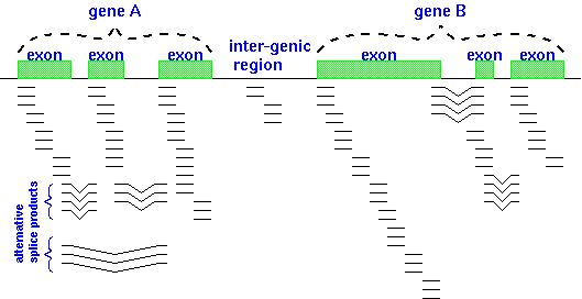
Another complication is shown in the figure below - alternative
splicing patterns. Transcriptomics (the study
of the transcriptome) is revealing that alternative splicing
occurs more frequently in eukaryotic gene expression than was
previously appreciated.
|
|
 |
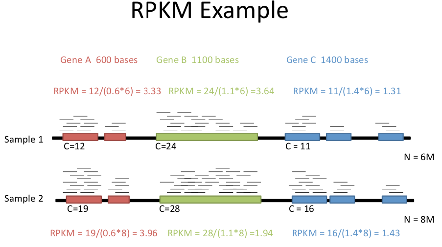
Another consideration of RNAseq methods is that since each read is the same length, but genes are different lengths, longer genes will be over-represented. Therefore, we need to correct reads for:
This makes results comparable across experiments. Depending on whether you are doing single reads or paired-end reads, there are two almost identical formulae.
RPKM = C / LN
Where: