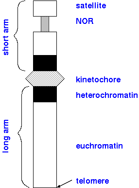
An ideogram of a metaphase chromosome.
The ability to study eukaryotic genomes depends upon the fundamental ability to uniquely identify each chromosome, and to detect changes in chromosome number and structure. Even something as fundamental as the number of chromosomes (2N) can be crucial, but may be hard to determine. For example, until the 1950s there were many independent observations leading to a human diploid complement of 2N = 48. As banding methods improved, the correct number of 2N = 46 was finally determined, and, upon reexamination of previous cytology, found to be supported by the evidence. This caused some embarrassment at the time. This illustrates the point that before you can even count chromosomes, you have to be able to uniquely identify them.
| The classification of chromosomes is based on
physical characteristics such as telomere, position of
kinetechore, secondary constrictions, size and position of
heterochromatic knobs and relative lengths of the
chromosomes. An ideogram of a metaphase chromosome. |
|
Karyotype - the exact chromosome complement of the organism. The karyotype is particular to an individual or to related groups eg. species.
Karyogram - the physical measurement of the chromosomes from a photomicrograph where the chromosomes are arranged in the descending order- longest to shortest. Different groupings are also possible.
Idiogram - a diagrammatic sketch or interpretative drawing of the chromosomes based on physical characteristics visible in the karyogram.
Karyotype analysis is usually based on somatic metaphase
chromosomes obtained after pretreatment.
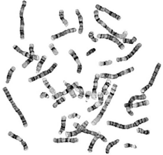
| Banding makes it easier to uniquely identify
specific chromosomes. G-banded chromosomes from a human male. From Cytogenetics Gallery, Department of Pathology, University of Washington Link here. |
 |
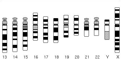
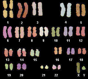
| However, since most genomes contain many
chromosomes, it is most instructive to arrange them in a
karyogram. In most organisms, the largest chromosome is
numbered as 1, and successive numbers assigned to
chromosomes in descending order of size. Karyogram of G-banded chromosomes from a human male. From Cytogenetics Gallery, Department of Pathology, University of Washington Link here. |
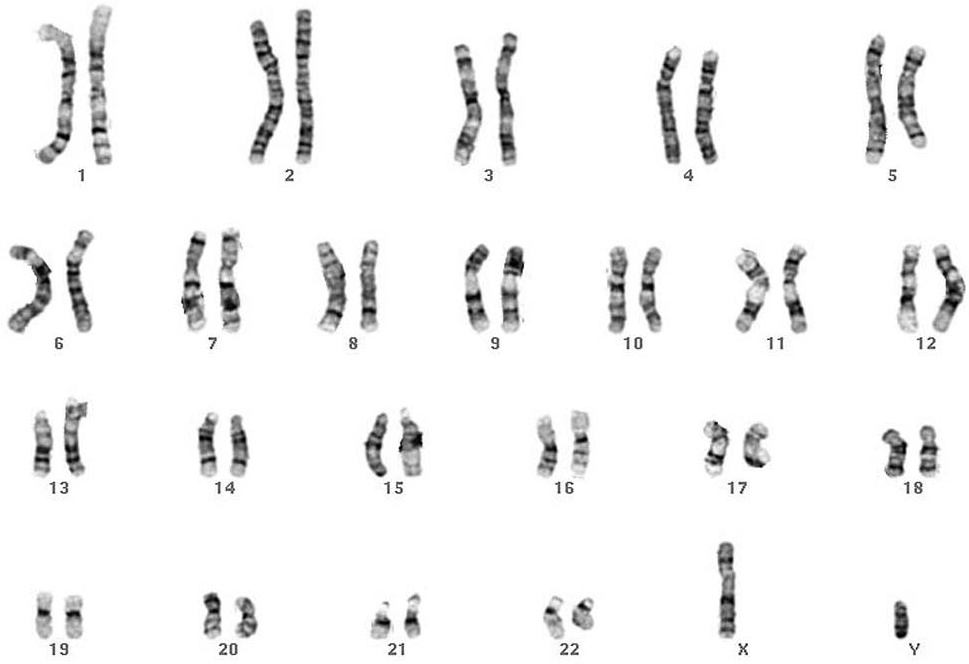 |
The karyogram accomplishes several things. First, it organizes
the chromosomes into homologous groups, making it easier to detect
nondisjunction. Secondly, comparison between banding patterns of
homologous chromosomes aids in the detection of chromosomal
aberrations such as deletions, insertions, or translocations. A
uniform nomenclature makes it possible to compare chromosome
structure among different individuals. Idiograms allow the
representation of most of the key features of chromosomes in a
standardized way.
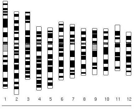 |
 Ideogram of human chromosomes. From Cytogenetics Gallery, Department of Pathology, University of Washington Link. |
Chromosome arms are defined with respect to the kinetochore. Although the terms "kinetochore" and "centromere" are used interchangeably in chromosome nomenclature, it is probably more correct to refer to kinetochore, since we don't really see the centromere, which is simply a DNA sequence. Rather, we see the proteinaceous kinetochore, and the distinct heterochromatic staining that occurs in the vicinity of the centromere.
Long arm (l) and short arm (s) is expressed as a ratio: l/s. These values have also been expressed as long arm (q) and short arm (p = "petite") in the study of human chromosomes and the arm ratio given as q/p.
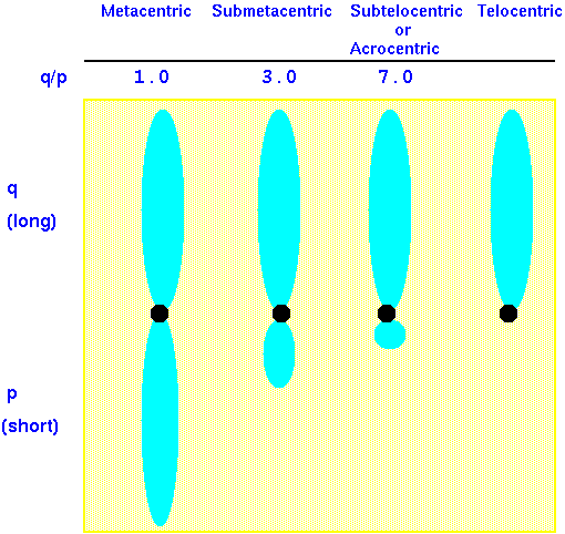
Note: There is no such thing as a truly telocentric chromosome. If the centromere were at the end of the chromosome, it would be lost in a few cell divisions (See lecture 12). The term 'telocentric' simply refers to the fact that the short arm of the chromosome, including its telomere, is so short that it can't be seen under the microscope.
Example:
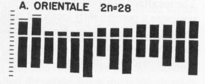
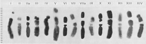
| Figure 5.4 Karyotype and idiogram of Geimsa N-banded chromosomes of barley | 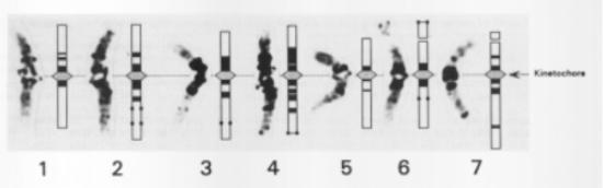 |
| Table 5.2. Relative Chromosome Arm Length (%), Mean Arm Ratio of Hordeum vulgare cv. Shin Ebisu (SE 16) | ||||||||||||||||
|---|---|---|---|---|---|---|---|---|---|---|---|---|---|---|---|---|
|
|
||||||||||||||||
| 1 | 2 | 3 | 4 | 5 | 6 | 7 | ||||||||||
| Cell no. | l | s | l | s | l | s | l | s | l | s | l | s | l | s | 6 Sat | 7 Sat |
| 1 | 7.69 | 7.69 | 9.23 | 6.92 | 9.23 | 6.15 | 7.69 | 6.92 | 7.69 | 5.38 | 7.69 | 4.61 | 8.46 | 4.61 | 2.30 | 1.53 |
| 2 | 7.69 | 8.09 | 8.90 | 7.29 | 9.72 | 6.47 | 8.90 | 5.67 | 7.29 | 4.85 | 7.29 | 4.04 | 9.72 | 4.04 | 2.42 | 1.62 |
| 3 | 6.98 | 6.98 | 9.56 | 8.08 | 8.46 | 6.61 | 8.08 | 6.99 | 7.35 | 5.15 | 6.61 | 4.42 | 9.56 | 5.14 | 2.20 | 1.47 |
| 4 | 8.43 | 7.23 | 8.43 | 7.23 | 9.04 | 6.62 | 7.83 | 6.63 | 7.23 | 5.42 | 7.23 | 4.21 | 9.64 | 4.82 | 2.41 | 1.80 |
| 5 | 8.41 | 7.96 | 8.85 | 7.52 | 8.85 | 6.19 | 7.08 | 6.19 | 7.08 | 5.31 | 7.08 | 4.42 | 10.62 | 4.42 | 1.77 | 1.77 |
| 6 | 7.14 | 7.93 | 9.52 | 7.14 | 9.52 | 6.74 | 7.93 | 5.95 | 6.74 | 4.76 | 7.14 | 4.37 | 9.92 | 5.16 | 2.38 | 1.58 |
| 7 | 7.41 | 7.41 | 9.05 | 6.58 | 9.47 | 6.58 | 7.41 | 6.58 | 7.41 | 4.94 | 8.23 | 4.94 | 9.05 | 4.94 | 2.47 | 1.65 |
| 8 | 6.36 | 7.07 | 9.19 | 7.06 | 9.89 | 7.06 | 7.77 | 7.36 | 7.77 | 5.65 | 7.42 | 4.24 | 9.54 | 4.59 | 2.82 | 2.12 |
| 9 | 7.64 | 7.64 | 8.92 | 7.32 | 9.55 | 7.01 | 7.64 | 6.37 | 7.64 | 5.09 | 7.01 | 4.45 | 8.92 | 4.77 | 2.22 | 1.27 |
| 10 | 8.62 | 7.66 | 8.62 | 6.71 | 8.62 | 5.75 | 7.66 | 6.70 | 7.66 | 5.75 | 6.70 | 3.83 | 10.92 | 4.78 | 1.91 | 1.91 |
| Mean | 7.64 | 7.57 | 9.03 | 7.19 | 9.24 | 6.52 | 7.80 | 6.44 | 7.39 | 5.23 | 7.24 | 4.36 | 9.64 | 4.73 | 2.29 | 1.67 |
| 95%
confidence
limit |
±0.51 | ±0.27 | ±0.26 | ±0.29 | ±0.34 | ±0.28 | ±0.34 | ±0.29 | ±0.23 | ±0.23 | ±0.34 | ±0.21 | ±0.53 | ±0.24 | ±0.21 | ±0.17 |
| Relative lengthb | 65.89 | 65.28 | 77.88 | 62.06 | 79.68 | 56.24 | 67.29 | 55.53 | 63.72 | 45.14 | 62.46 | 37.57 | 83.12 | 40.78 | 19.75 | 14.42 |
| 95% confidence limit | ±4.39 | ±2.34 | ±2.23 | ±2.56 | ±2.95 | ±2.48 | ±2.93 | ±2.56 | ±1.97 | ±2.04 | ±2.90 | ±1.85 | ±4.58 | ±2.07 | ±1.81 | ±1.48 |
| Arm ratio (l/s) | 1.01 | 1.26 | 1.42 | 1.21 | 1.41 | 1.66 | 2.04 | |||||||||
| Note: l = long arm, s =
short arm. a Arm ratios do not include satellite. b Based on 100 units for both arms of chromosome 6. From Singh, R.J. and Tsuchiya, T. 1982a. Theor. Appl. Genet. 64:13-24. |
||||||||||||||||
| Table 5.3. Comparison of Relative Chromosome Arm Length and Arm Ratios in Barley Observed by Several Authors | |||||||||||||||||||||
|
|
Arm ratio l/s |
|
Arm ratio l/s |
|
Arm ratio l/s |
|
Arm ratio l/s |
|
Arm ratio l/s |
|
Arm ratio l/s |
|
Arm ratio l/s | ||||||||
| Ref. | l | s | l | s | l | s | l | s | l | s | l | s | l | s | |||||||
| Tjio & Hagberg, | 78.4 | 58.5 | 1.34 | 71.7 | 61.1 | 1.17 | 63.7 | 58.6 | 1.09 | 67.2 | 51.8 | 1.30 | 60.7 | 44.3 | 1.37 | 62.1 | 37.9 | 1.64 | 78.5 | 32.2 | 2.44 |
| 1951 | 63.7 | 58.6 | 1.09 | 78.4 | 58.5 | 1.34 | |||||||||||||||
| Tuleen, 1973 | 64.5 | 61.3 | 1.05 | 75.0 | 60.5 | 1.24 | 74.5 | 56.8 | 1.31 | ||||||||||||
| Künzel, 1976 | 66.5 | 64.2 | 1.04 | 73.9 | 63.0 | 1.17 | 72.4 | 58.5 | 1.24 | 68.2 | 58.0 | 1.18 | 63.6 | 44.4 | 1.43 | 62.1 | 36.7 | 1.69 | 79.8 | 37.7 | 2.12 |
| Singh and Tsuchiya, 1982a | 65.9 | 65.3 | 1.01 | 77.9 | 62.1 | 1.25 | 79.7 | 56.2 | 1.42 | 67.3 | 55.5 | 1.21 | 63.7 | 45.1 | 1.41 | 62.5 | 37.6 | 1.66 | 83.1 | 40.8 | 2.04 |
| From Singh, R.J. and Tsuchiya,
T. 1982a. Theor. Appl. Genet. 64:13-24. |
|||||||||||||||||||||
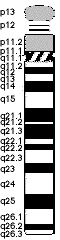
In human and other genomes, chromosomes are broken down into arms, p & q, regions, and bands. This is illustrated on human chromosome 15. The following rules apply:
The nucleolar organizing region (NOR) is the site of ribosomal RNA genes. Usually, rRNA genes are tandemly-repeated in a hundred or more copies at a small number of NOR loci on several chromosomes. The NOR forms during chromosome decondensation in telophase. Since it contains rRNA genes it serves as the site of rRNA synthesis by RNA polymerase I. This region appears as a secondary constriction (the kinetochore or centromere being the primary constriction) on certain chromosomes in the genome. The NOR is not a true constriction and is actually the same diameter as the rest of the chromosome. It appears as a constriction because it does not pick up stain. The lack of staining at the NOR makes the remaining portion of the chromosome above the NOR appear to be removed from the rest of the chromosome as a chromosome fragment or satellite.
Each species has one or more homologous pairs with an NOR. Often each basic genome has a pair of satellite chromosomes. Satellites can serve as markers of basic genomes and are therefore valuable for taxonomic studies. Satellites are heterochromatic and can vary considerably in size.
Specific hybridization probes can be made for each chromosome, allowing karotyping by "chromosome painting".
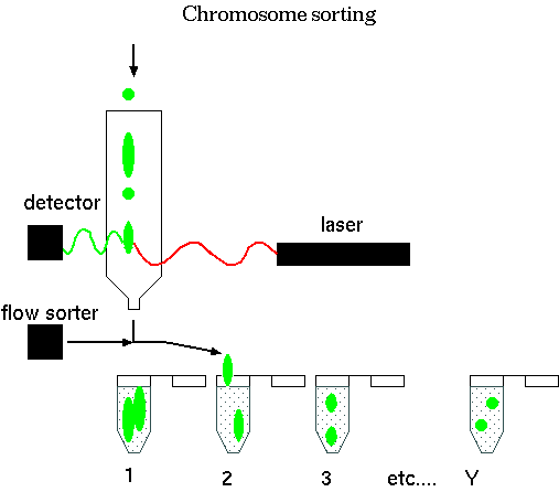
When chromosomes are fluorescently-tagged, the amount of fluorescence is proportional to the size of the chromosome. Flow cytometers (Fluorescence-activated cell-sorters) illuminate chromosomes with a laser, and the amount of fluorescence is detected. Depending on the intensity, a chromosome leaving the sorter is deflected into a particular tube. The result is that all 24 human chromosomes can be purified. By PCR with random primers, the entire DNA complement of a given chromosome can be amplified, to produce small samples of DNA from a single chromosome.
Since most of the human genome is repetitive DNA, total chromosomal DNA from any one chromosome would be expected to hybridize with all chromosomes. On the other hand, low copy number sequences from each chromosome should be unique to that chromosome. To saturate repetitive chromosomal sequences during Fluorescence In-situ hybridization (FISH), chromosomes can be hybridized with non-labeled probe from repetitive DNA, leaving only low-copy number sequences unhybridized. The low copy sequences are free to hybridize specifically with low-copy sequences from the probe. Blocking probe is made by allowing unlabeled total human DNA to anneal to C0 t = 1, at which low-copy DNA will remain single-stranded, but repetitive DNA will be in duplex form. Single-stranded DNA can be separated from double-stranded DNA by HAP chromatography. For some species, C0t1 DNA is commercially available.
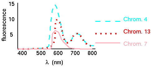
Because there are 24 human chromosomes (counting X & Y), and only a few dyes available for fluorescent labeling, each chromosome must be labeled with a unique combination of dyes so that a distinct emission spectrum will be obtained for each chromosome. Typically 5 dyes are used: Cy2, Spectrum Green, Cy3, Texas Red and Cy5. For 5 dyes, there are 25 = 32 possible combinations. Thus, a probe made with only 1 dye might have a single peak emission wavelength, while a probe made with 3 dyes might have peaks at 3 distinct wavelengths. By measuring the emission spectra at each pixel in the image of the chromosomes, visualized in fluorescence microscopy, a computer program can determine which chromosome-specific probe produced that pixel.
FISH is performed using a mixture of the 24 chromosome-specific probes, and a large excess of blocking probe. Although the labeled chromosome-specific probes also contain repetitive sequences, the repetitive sequences on the slide are saturated by unlabeled probe, allowing very little of the labeled repetitive sequences to hybridize. Consequently, only low-copy number labeled sequences will be unblocked on the slide, and only chromosome specific sequences will hybridize. The chromosomal image is acquired by a CCD camera, and a computer program determines the emission spectrum for each pixel. Based on the spectrum, that pixel is assigned a color for classification purposes, resulting in an image that shows each chromosome to be a distinct color. As we will see in Lecture 19, chromosome painting makes it easy to detect chromosomal abnormalities, such as translocations, deletions, or inversions.
For further reading consult: Schröck, E. et al. (1996) Multicolor spectral karyotyping of human chromosomes. Science 273: 494-497.