A common issue in the electromagnetic inverse scattering community is the lack of open access measurement data from experimental laboratory set-ups or prototype systems. Data available from the Ipswich (e.g. McGahan and Kleinman, [1, 2]) and Fresnel (e.g. Geffrin and Sabouroux, [3, 4]) databases have addressed this insufficiency. These data were collected with a bi-static, mechanically scanned system with antennas located in the far-field. However, there are many applications, such as biomedical imaging or non-destructive testing, for which scattering data are better collected with a mechanically static near-field system. Advantages of near-field imaging include higher resolution, but additional complications such as antenna coupling and a complicated incident field do occur. We are aware of only one repository of near-field multi-static data (Mallorqui et. al. [5]), but this dataset is available pre-calibrated, with closely coupled antennas removed, and only for a single frequency.
With the goal of stimulating research with respect to near-field multi-static imaging calibration and inversion, we present a database of microwave scattering measurements. All of the measurement data are presented uncalibrated. The measurements were taken with the imaging system outlined in a previous publication (Gilmore et. al, [6]). Targets were elongated in the z-direction, and the linearly polarized antennas were oriented in the same direction. Thus we intend for the 2D Transverse Magnetic (scalar) approximation to apply. Several dielectric and metallic targets were interrogated in free-space under two different schemes labeled tomographic and radar. The tomographic data are multi-static (i.e. S_{a,b}) in the frequency range of 3 to 6 GHz in 0.5 GHz steps, and the radar data are reflection data only (i.e. S_{x,x}) for 1601 linearly spaced frequencies from 3 to 10 GHz.
The microwave imaging system used to collect the EIGOR data is fully described in [6]. A photograph of the system and a close-up of the antenna as well as two schematics of the chamber are shown in the figures. The system consists of 24 double- layer vivaldi antennas (DLVAs), supported inside a Plexiglas imaging chamber. The antennas have an operating bandwidth from 3 to 10 GHz (stipulated as the continuous frequency range for which S11 is below -10 dB). A detailed description of the antennas can be found in [13,14]. Additional behaviour of the antennas when co-resident in the chamber is available in [6].
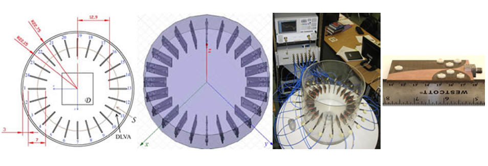
The microwave transmitter/receiver consists of a two-port Agilent 8363B PNA-Series Vector Network Analyzer (VNA). The VNA is connected to the antennas with a 2x24 cross-bar mechanical switch (Agilent 87050A-K24), which provides isolation of greater than 95 dB over the frequency range of interest. The exterior Plexiglas cylinder has an inner radius of 22.2 cm. Each Vivaldi antenna is 7 cm long, and the base is held 3.0 cm from the wall by the connectors. Thus, the tip of the antenna is located 10 cm from the edge of the wall, and the maximum imaging domain, D, consists of a circle of radius 12.9 cm, located at the center of the chamber. If a square domain is used, the maximum size is a length of approximately 18 cm. In practice, we have used an imaging domain, D of 12 cm sides, and all targets are inside the 12x12 cm imaging domain. During data collection, the chamber was surrounded by radar absorbing material (RAM).
Data were collected for two metallic cylinders. The cylinders are shown at the right. Metallic cylinder #1 is a hollow steel cylinder with an outer diameter of 2 inches (d = 5.08 cm) and a length of 65 cm. Metallic cylinder #2 is an aluminum cylinder with an outer diameter of 3.5 inches (d = 8.89 cm), and a length of 46 cm. For both metallic cylinder datasets, the cylinders were centered in the chamber, and no other targets were present.
There are three different nylon targets used in the EIGOR data. Nylon-66 was used, and the permittivity values are available in the appendix of [16]. At 3 GHz, the dielectric constant is expected to be eps_r = 3:03 + j0:03. Three different cylinders were used: a large cylinder with a diameter of 4 inches (d = 0.16 cm) and a length of 50 cm, and two smaller cylinders with a diameter of 1.5 inches (d = 3.81 cm) and a length of 44 cm.
Three sets of scattering parameters were collected with these cylinders. `Nylon #1' consists of the large 4 inch diameter cylinder centered in the chamber. `Nylon #2' consists of a single 1.5 inch diameter cylinder in the center of the chamber. For the third experiment `Two Nylon Cyl.', consists of two 1.5 inch diameter cylinders, placed 0.5 cm apart. A photograph of these cylinders in the imaging chamber is shown below.

Geometrically, the most complicated target is the e-phantom. A photograph and schematic with dimensions in cm are shown below. The phantom was constructed from ultra-high molecular weight polyethylene, which has an expected dielectric constant of eps_r = 2:3 @ 5 GHz, with negligible loss [17].

The wood and nylon phantom is shown below. The phantom consists of a 1.5 inch diameter nylon-66 cylinder next to a wood block of dimensions 8.7x 8.8 cm and a height of 31 cm (the block is an untreated spruce `4 x 4' wood construction post). The permittivity of the wood was measured via our Agilent 85070 open-ended coaxial probe kit from 0.2 to 8.5 GHz, and the values are presented in the Figure below.


For the tomographic and radar datasets, we have measurements for 6 lossless targets, plus two empty chamber (incident field) measurements. The incident field measurements were taken as the first and last datasets. Comparing the two can provide an estimate of the noise associated with the system. All data are `total field' measurements. Thus, to obtain scattered field S-parameters for a particular target, one of the incident field measurements must be subtracted. During data collection, the VNA was calibrated to its own ports. Thus, the effects from the cables between the VNA and switch, the internal paths of the switching matrix, and the cables from the switch to the antennas (plus associated connectors) are in the measurement. These effects are readily removed via a scattered field calibration.
For each target, two datasets were collected. These datasets are labeled tomographic and radar. The target was in the same physical position for both measurements, and all efforts were made to keep cables stationary throughout the entire measurement process. The tomographic datasets consist of measurements from 3 to 6 GHz in 0.5 GHz steps, with 24x23 transmission measurements of S_{a,b}, (reflection measurements, S_{x,x}, are excluded from these data).
For lossy targets, we have also included a measurement of a wood-nylon phantom, plus associated incident and metallic cylinder data. Data were collected for frequencies of 3-10 GHz in 1 GHz steps. These data are only in the tomography format. These data were collected on a different day with an older version of the data collection software, and are thus presented separately. Calculation of scattered parameters as well as calibration should stay within the particular tomography dataset.
In general, the raw data for the tomographic measurements are not reciprocal. That is, S_{a,b} does not equal S_{b,a}. For ease of implementation, we have utilized a single transmitter from the VNA, and when this is done, the internal paths in the switch are not the same length for the two scenarios. For example, when transmitting from port `a' and receiving on port `b', the total path length in the switch is different than receiving on port `a' and transmitting on port `b'. This difference primarily affects the phase of the raw measurement, and can be removed via calibration.
All data are presented in a raw, uncalibrated format. While one of the purposes of this database is to encourage calibration research, we provide our most commonly used calibration method here.
There are two main purposes of calibration: (i) to convert the S_{a,b} values measured by the VNA into field values (u = E_z) used in the inversion algorithms, and (ii) to eliminate/compensate for modeling error and other errors. We define modeling error as arising from any mismatch between the assumed computational model and the physical measurement system (e.g., a 2D scalar Green's function vs. physical 3D vector wave propagation).
To perform the calibration, we first measure scattered data from a known cylinder placed in the centre of the chamber. Typically, we use a metallic cylinder, but other objects are also possible. We denote these S parameters as S^sct,known_{a,b} . Next, we consider the S parameters from the object we wish to image (e.g., the e-phantom) and we denote these S parameters as S^sct,unknown_{a,b} . Assuming a 2D line source generated incident field, we calculate the analytic scattered fields (under the 2D TM assumption) from the known object, and label them u^sct,known. These values are easily calculated analytically for metallic or dielectric cylinders [16]. Finally, the calibrated measured fields for the unknown target are calculated by

The process is repeated independently for every transmit/receive pair. This method of calibration will eliminate any errors which are constant over the two measurements (S^sct_{a,b} known and unknown). Examples of these types of `removable' errors include cable losses and phase shifts, or mismatches at connectors. However, there are other factors in the measurement which are not constant between the two measurements, and thus not entirely removed via the above calibration method. For example, the antenna factor is not guaranteed to be the same for the known and unknown measurements (as the system is operating in the near-field). Another error which is not entirely compensated for is the antenna coupling, as the coupling will change when different scatterers are present in the chamber. For these reasons, we expect that the known calibration object should be as similar as possible to the expected class of unknown targets.
The microwave tomography data found here is provided with the understanding that it will be used for research purposes by the research community. If you use any of this data for results in your future publications we would appreciate it if you reference our publications wherein this data and MWT system are described. These papers can be found in the References Section of this web site. For the actual data, there is a conference presentation where we announced the availability of this data and we have submitted a detailed description to the Inverse Problems journal. In particular, for the data description, please refer to:
Colin Gilmore, Amer Zakaria, Puyan Mojabi, Majid Ostadrahimi, Stephen Pistorius, Joe LoVetri "A 2D Near-Field Multi-Static Wideband Microwave Scattering Repository for the Testing of Calibration and Inversion Algorithms," IEEE Int. Symp. on Ant. and Prop. and USNC/URSI National Radio Science Meeting, Spokane, Washington, USA, 3-8 July, 2011.
Colin Gilmore, Amer Zakaria, Puyan Mojabi, Majid Ostadrahimi, Stephen Pistorius, Joe LoVetri "The University of Manitoba Microwave Imaging Repository: A Two-Dimensional Microwave Scattering Database for Testing Inversion and Calibration Algorithms [Measurements Corner]," IEEE Antennas and Propagation Magazine, vol.53, no.5, pp.126-133, Oct. 2011. doi: 10.1109/MAP.2011.6138442
For tomographic dataset #1, listed in Table 1, the general format is in 7 columns. In order, these describe the frequency of operation (in GHz), the transmitter number (1-24), the receiver number (1-24), two columns of zeros, real part of S_{a,b} for the transmit/receive pair, and imaginary part of S_{a,b}. The two columns of zeros may be ignored: these columns are intended to record the elevation and angle of a positioning motor [15], which was not used for these data. For the lossy target tomographic dataset #2, listed in Table 2, the general format is in 5 columns. The order is the same as the previous tomographic dataset, but with the two columns of zeros removed. For the radar dataset, listed in Table 3, the general data format is in 4 columns: frequency (in GHz), antenna number (x), real part of S_{x,x} and imaginary part of S_{x,x}.
| Target Name | File Name | |
|---|---|---|
| Non-calibrated | Calibrated | |
| Incident 1 | tomographic_incident.txt | |
| Incident 2 | tomographic_incident_2.txt | |
| Metal cyl. #1 | tomographic_metal_2p0_inch_diam.txt | tomographic_metal_2p0_inch_calibrated.txt |
| Metal cyl. #2 | tomographic_metal_3p5_inch_diam.txt | |
| Nylon cyl. #1 | tomographic_nylon_4p0_inch_diam.txt | tomographic_nylon_4p0_inch_calibrated.txt |
| Nylon cyl. #2 | tomographic_nylon_1p5_inch_diam.txt | tomographic_nylon_1p5_inch_calibrated.txt |
| Two nylon cyl. | tomographic_nylon_cyls_0p5cm.txt | tomographic_nylon_cyls_0p5cm_calibrated.txt |
| e-phantom | tomographic_e_phantom.txt | tomographic_e_phantom_calibrated.txt |
| Target Name | File Name |
|---|---|
| Incident | incident_3.txt |
| Metal cyl. (3.5 inch) | metal_3p5_inch_diam.txt |
| wood and nylon | wood_and_nylon_diel.txt, wood_and_nylon_calibrated |
| Target Name | File Name |
|---|---|
| Incident 1 | radar_incident.txt |
| Incident 2 | radar_incident_2.txt |
| Metal cyl. #1 | radar_metal_2p0_inch_diam.txt |
| Metal cyl. #2 | radar_metal_3p5_inch_diam.txt |
| Nylon cyl. #1 | radar_nylon_4p0_inch_diam.txt |
| Nylon cyl. #2 | radar_nylon_1p5_inch_diam.txt |
| Two nylon cyl. | radar_nylon_cyls_0p5cm.txt |
| e-phantom | radar_e_phantom.txt |
[1] R. McCahan and R. Kleinman, "Special session on image reconstruction using real data," IEEE Antennas and Propagation Magazine, vol. 38, no. 3, p. 39, June 1996.
[2] R. McGahan and R. Kleinman, "Third annual special session on image reconstruction using real data, part 1," IEEE Antennas and Propagation Magazine, vol. 41, no. 1, pp. 34-36, 1999.
[3] J.-M. Gefferin, P. Sabouroux, and C. Eyraud, "Free space experimental scattering database continuation: experimental set-up and measurement precision," Inverse Problems, vol. 21, pp. S117-S130, 2005.
[4] A. Litman and L. Crocco, "Testing inversion algorithms against experimental data: 3D targets," Inverse Problems, vol. 25, p. 020201, 2009.
[5] J. J. Mallorqui, N. Joachimowicz, J. C. Bolomey, , and A. P. Broquetas, "Database of `in-vivo' measurements for quantitative microwave imaging and reconstruction algorithms available," IEEE Antennas and Propagation Magazine, vol. 37, no. 5, pp. 87{89, 1995.
[6] C. Gilmore, P. Mojabi, A. Zakaria, M. Ostadrahimi, C. Kaye, S. Noghanian, L. Shafai, S. Pistorius, and J. LoVetri, "A wideband microwave tomography system with a novel frequency selection procedure," IEEE Transactions on Biomedical Engineering, vol. 57, no. 4, pp. 894-904, April 2010.
[7] C. Gilmore, P. Mojabi, A. Zakaria, S. Pistorius, and J. LoVetri, "On super-resolution with an experimental microwave tomography system," Antennas and Wireless Propagation Letters, IEEE, vol. 9, pp. 393-396, 2010.
[8] C. Gilmore, P. Mojabi, and J. LoVetri, "Comparison of an enhanced Distorted Born iterative method and the multiplicative-regularized contrast source inversion method," IEEE Transactions on Antennas and Propagation, vol. 57, no. 8, pp. 2341- 2351, August 2009.
[9] P. Mojabi and J. LoVetri, "A pre-scaled multiplicative regularized Gauss-Newton inversion," IEEE Transactions on Antennas and Propagation, vol. 59, no. 8, pp. 2954-2963, 2011.
[10] A. Zakaria, C. Gilmore, and J. LoVetri, "Finite-element contrast source inversion method for microwave imaging," Inverse Problems, vol. 26, p. 115010, 2010.
[11] P. Mojabi, J. LoVetri, and L. Shafai, "A multiplicative regularized Gauss-Newton inversion for shape and location reconstruction," (accepted) IEEE Transactions on Antennas and Propagation, vol. 59, 2011.
[12] C. Gilmore, A. Zakaria, P. Mojabi, M. Osadrahimi, S. Pistorius, and J. LoVetri, "A 2D near-field multi-static wideband microwave scattering repository for the testing of calibration and inversion algorithms," in 2011 IEEE Antennas and Propagation Society International Symposium and URSI National Radio Science Meeting, 2011.
[13] M. Ostadrahimi, S. Noghanian, L. Shafai, A. Zakaria, C. Kaye, and J. LoVetri, "Investigating a double layer vivaldi antenna design for fixed array field measurement," International Journal of Ultra Wideband Communications and Systems, vol. 1, no. 4, pp. 282-290, 2010.
[14] M. Ostadrahimi, S. Noghanian, and L. Shafai, "A modified double layer tapered slot antenna with improved cross polarization," 13th International Symposium on Antenna Technology and Applied Electromagnetics (ANTEM), Banff, Alberta, Canada, February 15-18, 2009.
[15] C. Kaye, C. Gilmore, P. Mojabi, D. Firsov, and J. LoVetri, "Development of a resonant chamber microwave tomography system," in Ultra-Wideband, Short Pulse Electromagnetics 9, F. Sabath, D. Giri, F. Rachidi, and A. Kaelin, Eds, Springer New York, 2010, pp. 481-488.
[16] R. Harrington, Time-Harmonic Electromagnetic Fields. New York: IEEE Press, 2001.
[17] W. S. Bigelow and E. G. Farr, "Impulse propagation measurements of the dielectric porperties of several polymer resins," AFWL Measurement Notes, Note 55, pp. 1-52, 1999.
Electromagnetic Imaging Laboratory at University of Manitoba. All rights reserved.