NonpaR: Nonparametric Statistical Tests
(Hollander and Wolfe, 1999)
The NonpaR module in MeV consists of four nonparametric tests that can be used to analyze several common experimental designs. Three of these tests, Wilcoxon Rank Sum, the Kruskal Test, and the Mack-Skillings Test find genes that are differentially expressed between two or more experimental groups under study. The Fisher Exact Test is applied to data where there are two distinct experimental groups and the data values for each gene are separated into two distinct bins using a numerical cutoff. The test then describes if a data bin (e.g. values above a supplied expression threshold) are over represented in one sample group or the other. Hollander and Wolfe provide a complete description of all of the methods in this module as well as the qualities and the general benefits of nonparametric statistical tests. Please refer to that text for a complete overview of nonparametric tests and the formulae for computing these test statistics.
Nonparametric tests make few assumptions about the underlying distributions of values in the population from which the sample is taken. There is no assumption that the population has a normal distribution of values. Note that there is assumed to be an underlying distribution and that different experimental groups are sampling populations that share the same distribution type. The difference from parametric tests is that the underlying distribution is not necessarily assumed to be normal. In addition to their distribution-free property, nonparametric tests also tend to be less sensitive to outlier measurements than their parametric counterparts since nonparametric tests are based on the ranking of the data.
Brief Test Descriptions
The test handles an experimental design where there are exactly two experimental groups and there are replicate hybridizations for each of these groups. The null hypothesis is that the observations for both samples come from the same probability distribution, that the underlying population means are the same. The test attempts to reject this hypothesis and reports genes that are over or under (two-tailed test) expressed in group 2 relative to group 1.
The is analogous to the parametric one-way ANOVA test. This test handles designs where there are n-experimental groups that vary in some way related to one experimental factor. An example might be three experimental groups representing sets of patients in a clinical trial, ‘control-untreated’, ‘low dose intervention’, and ‘high dose intervention’. The Kruskal tests can be applied to two or more experimental groups. If there are exactly two groups then the Wilcoxon Rank Sum test is typically used.
The is a generalization of the more familiar Friedman test for two factor designs. This test handles design where there are two experimental factors (such as strain and treatment) and there are some number of levels of each factor (e.g. 2 strains and 3 treatment levels, as in a 2 x 3 design). Unlike the Friedman test, the Mack-Skillings test allows for replication and handles balanced or unbalanced complete designs. This means that each factor combination group should have one or more observation but that factor combination groups (or different cells in the design matrix) can have uneven numbers of replicates. The following table provides an example of an unbalanced complete design having at least one observation per strain/temperature combination but having uneven numbers of replicates across strain/temperature combinations. Two factor design table example: (numbers represent the number of samples in each experimental group)
| Strain | Temp = 25C | Temp = 32C | Temp = 37C |
| Wild Type | 4 | 4 | 3 |
| Mutant A | 3 | 3 | 4 |
The test looks for differences between groups that are related to either of the two factors.
The is applied to data where there are two distinct groups of samples and the data can be binned into two groups, called data bins, based on a supplied numerical cutoff. The test then answers the question as to whether there is a non-random association between a sample group and the binned data. Stated in a more another way the question may be asked, are the data values in data bin one associated disproportionately with sample group one or sample group 2? A concrete example of this is where the input data values are from CGH and the data values are numerical representations of absent/present calls (0 or 1) and the samples fall into two distinct groups such as patient set A and patient set B. A contingency matrix classifies each data value for a particular gene according to this sample table:
| Patient Set A | Patient Set B | |
| Present Calls | 16 | 4 |
| Absent Calls | 2 | 19 |
Patient set A has 18 members, patient set B has 23 members. For this particular gene, there are present calls for 16 of 18 patients in set A while in set B there are only 4 present calls out of 23 patients.
This contingency matrix captures the disproportionate number of present calls in patient set A (there are other ways to express the disproportionality). The Fisher Exact Test takes this matrix and reports a p-value describing the probability of this matrix and less likely (more disproportionate situations) occurring by chance. One tailed probabilities are reported for situations where the expected disproportionality is in one direction or the other. Most users will be most interested in the two tailed probability in which reports the probability of having a disproportionality reflected in the matrix in either extreme.Running NonpaR Tests
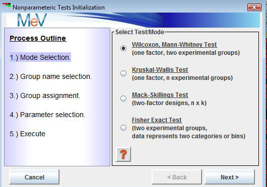
NonpaR uses a set of parameter input dialogs that open sequentially to provide input options that correspond to each step of the process. The first step in the processes is the selection of a test or mode. The test descriptions above will help determine which tests would fit your experimental design and address the specific hypothesis to be tested. The Wilcoxon and Kruskal tests progress using similar input dialogs while the Mack-Skillings test uses parameter panels that support two factor experimental designs. For that reason we first describe the more basic Wilcoxon and Kruskal input process and then turn to the dialogs specific to running the Mack-Skillings test. The Fisher Exact Test will follow.
Wilcoxon Rank Sum and Kruskal Tests
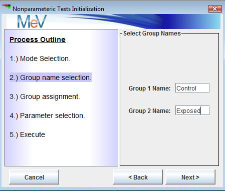
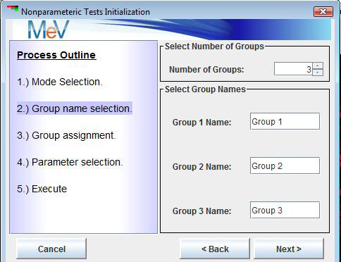
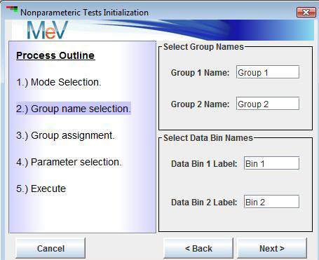
The second step is to specify group names or labels. By default, all tests start with the names initialized as group1, group2…etc.. These can be modified to reflect the conditions related to each experimental group. In the case of the Kruskal test, the number of groups is selected in addition to the group labels (See figures below).
ParametersAlpha Value
The alpha value is a p-value cutoff. p-values below this value are considered as justification for rejection of the test's null hypothesis. Lowering the alpha value, or critical p-value, makes the test more stringent by limiting chance of a single type two error.
FDR: False Discovery Rate (when available)
The False Discovery Rate (FDR) reports an estimate of the fraction of false positives among a set of genes called signficant. This option uses the Benjamini-Hochberg correction which is described as a correction on the p-value such that the FDR for the collection of genes with p-values less than a particular gene i, is less than the corrected p-value for gene i. The FDR estimates the number of false positives such that if you call 100 genes positive and the FDR is 0.05 then it is estimated that 5 genes or fewer are falsely called significant.
There are two options for FDR, one in which you supply and FDR prior to the analysis, and a second option that supports a user interface to permit balancing the number of significant calls with FDR following computation of the results. This second option presents a graph of FDR vs. number of significant genes.
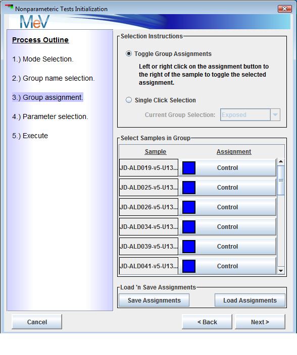
The third step is group assignment where each sample is assigned to a specific experimental group or placed into a group that is excluded from the current run. Left clicking on an assignment button next to a sample will change the group assignment to the next group. Successive left clicks will cycle forward through the possible group assignments. The buttons have been modified so that a right click will cycle through the group options in the reverse order which can be useful in the case where there are multiple groups. Another option is to use the Single Click Selection option.
Select a particular group to assign from the dropdown menu and then left click on assignment buttons next to the samples that fall into the selected group. Note that after group assignments are made that a file can be saved that captures the group assignments. This can be loaded on future runs to specify group assignments.Step four is parameter selection. For the Wilcoxon and Kruskal tests this dialog present two possible criteria for controlling error rates when collecting ‘significant’ genes. The first is to supply an alpha value or critical p-value as a cutoff. The other option is to use an estimated FDR or false discovery rate. This attempts to estimate the fraction of false positives among the set of genes selected by the test. Under the FDR option one can either select to enter a specific FDR cutoff or can use an interactive graph to adjust the relationship between number of genes captured and the estimated FDR for that group of genes. The FDR option to control type I errors uses the Benjamini-Hochberg (BH) Correction of p-values and ranks based on these adjusted p-values.
In all cases the raw p-values are reported and in the case of FDR, the BH adjusted p-values are also reported.If the FDR option is selected, an interactive graph is displayed to allow the user to adjust the number of captured genes while observing the FDR. The graph, shown in the figure below allows the user to zoom in to view the more critical behavior below FDR’s of 0.1. Each zoom step increases or decreases the displayed upper end of the FDR range according to these preset levels, 1.0, 0.5, 0.25, 0.1, 0.05. The lower limit is kept at zero. Adjustments to the FDR cutoff can be made in 0.01 unit increments. The lower portion of the window displays the number of genes captured and the estimated FDR for that set of genes and the number of genes that the FDR represents.
The output from NonpaR consists of the typical cluster viewers, Expression Images, Expression Graphs, Centroid Graphs, and Table Viewers. The Cluster Info viewer will capture the number of significant genes, the test name, and the significance criteria and value. One important note is that clusters saved to file from any of the NonpaR cluster viewers will have the measured statistic and p-values output to the file in addition to the expression and annotation information.
Mack-Skillings (MS) Test Dialogs
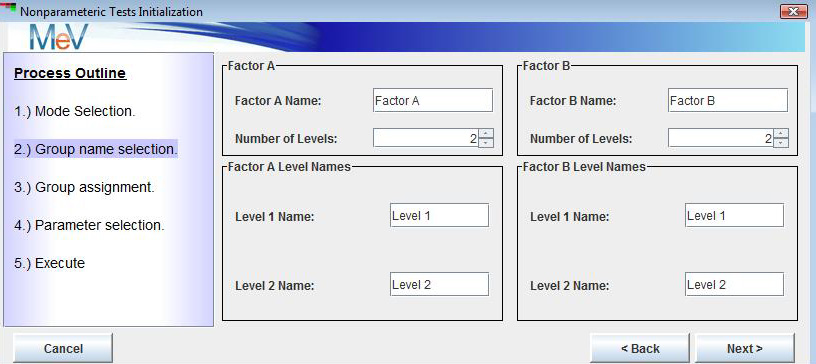
After selection to run MS a dialog will be presented that will capture some information regarding the experimental design. This dialog, pictured below, captures labels (names) for the two factors being studied. By default the factor labels are initially labeled as Factor A and Factor B but one can optionally change these to the actual factor names under study.
Buttons also allow one to select how many levels there are of each factor. For instance, if the first factor is strain and there are three strains being studied, select three. The same sort of selections are made for the second factor. The figures below show a 2 x 3 design, 2 strains by 3 growth media conditions. This dialog also permits the entry of meaningful names for each factors level. The initial default labels are Level 1, Level 2, etc..After specifying factor names, number of levels, and level names, select the button to open a two factor group selection dialog. Note the experimental design grid displayed in the upper portion of the dialog. If this doesn’t reflect the experimental design, select the button to make new selections. This dialog is used to assign samples to experimental groups represented in the design grid. Select the sample name in the table below by pressing the left mouse button while over the bold rectangle.
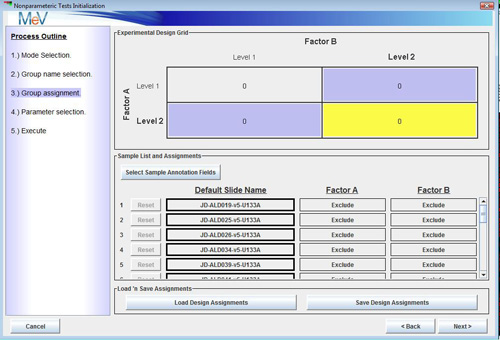
Two Factor Group Assignment Dialog. Samples are assigned to an experimental group in the design grid.
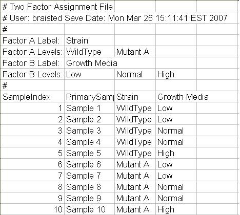
Group assignments can be saved to a file that can be reloaded to supply labels and map the samples to their respective groups.
The parameter selections in the final dialog provide an input field for the alpha value or critical p-value cutoff. The output, as mentioned previously for all NonpaR algorithms are the standard cluster viewers.
Fisher Exact Test
The Fisher Exact Test has some unique dialogs or parameters that must be selected as describe in this section. During execution of the tests, the data is divided first into one of two experimental groups (sets of hybridization results or columns in the expression matrix) and then the data values are partitioned using a numerical cutoff. This partitions the data values for each gene into the contingency matrix described and shown in the overview section on this tests.
The group name section dialog (shown below) includes two extra fields that are used to label the data bins that are partitioned based on the numerical cutoff (specified in a later dialog).
The next dialog to be displayed is used to assign each the loaded samples into one of the two experimental groups by clicking on the assignment buttons to the right of each sample label. This is the same dialog used for sample assignments for the Wilcoxon Rank Sum test shown in an earlier section.
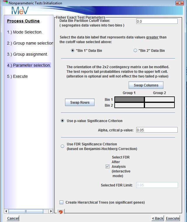
The final dialog captures the data bin cutoff value, the data bin label that should be associated with each data bin, the orientation of the 2x2 contingency matrix, and the various significance criteria options (alpha value or FDR).
The data bin cutoff value is to partition the data based on whether the data falls below or equal or greater than the supplied values. This is most often applied to data were the numerical values are either discrete numerical Present/Absent calls or where it makes sense to partition the data according to a supplied numerical cutoff. A concrete example the application of this test to CGH data, either raw values where a cutoff has been previously determined, or where the data consists of discrete absent/present calls.The next pair of buttons down on the dialog determine which of the supplied data bin labels should be associated with the data bin representing the values greater than the cutoff value.
The contingency matrix arrangement is displayed and allows the rows and columns to be swapped.
Note that for a particular gene, swapping rows and/or columns, simple places the count (number of data values) placed in each matrix cell in a different location in the matrix. The two tailed result, where the test for non-random association between the two factors is the focus, the arrangement of the matrix is not important. The one tailed test will report the disproportionality of the upper left matrix entry. The lower or left tail will indicate when relatively small counts are in the upper left cell while the upper tail or left tail will indicate when relatively large counts are in the upper left cell. The tail probabilities are the same regardless of orientation of the matrix but rather the left and right tail probabilities can be swapped depending on the orientation. Segregation of the significant two tailed results into two groups that are more significant on one tail or the other will illustrate the information gained from the one tailed result and how it relates to the combination of factors falling in the upper right cell.The output clusters from the Fisher Exact Test are split into significant and non-significant genes lists. The significant gene list also has two additional views, one containing those genes that are significant on the upper tail and another containing genes that are significant toward the lower tail. These tail views show the two directions of disproportionality. Note that one additional table view is created that reports the results of all genes that entered the analysis in one table. This cluster view can be saved to file using the right click ‘Save Cluster…’ menu option to capture the p-values for all genes being tested.
Data Bin Partition Value
Fisher Exact (FE) requires that the data fall into two bins. Usually these are CGH absent/present calls using discrete data or if an expression value can be used as a cutoff, the input data can be essentially continuous. The data bin partition splits that data by classifying each value as above the cutoff of below or equal to the cutoff.
The next to buttons allow you to associate one of your data bin names with the values that are greater than the supplied cutoff.
Contingency Matrix Orientation
The 2x2 contingency matrix that holds information indicating which values in an expression vector fall under a particular sample group and data bin, can have its columns and rows swapped. Note that this has no impact on the reported p-values but rather is used to describe the observed effect if a user is interested in a one-tailed result.
In most studies one is generally going to look for disproportionality where a data bin is over represented in one sample group or the other. In some cases, it might be more important to ask a more specific question such as which genes are over represented in sample group A. The comparison that is of greatest interest should appear in the upper left quadrant of the contingency matrix. The one tailed result will be focused on reporting on this observation.
Alpha Value
The alpha value is a p-value cutoff. p-values below this value are considered as justification for rejection of the test's null hypothesis. Lowering the alpha value, or critical p-value, makes the test more stringent by limiting chance of a single type two error.
FDR: False Discovery Rate
The False Discovery Rate (FDR) reports an estimate of the fraction of false positives among a set of genes called signficant. This option uses the Benjamini-Hochberg correction which is described as a correction on the p-value such that the FDR for the collection of genes with p-values less than a particular gene i, is less than the corrected p-value for gene i. The FDR estimates the number of false positives such that if you call 100 genes positive and the FDR is 0.05 then it is estimated that 5 genes or fewer are falsely called significant.
There are two options for FDR, one in which you supply and FDR prior to the analysis, and a second option that supports a user interface to permit balancing the number of significant calls with FDR following computation of the results. This second option presents a graph of FDR vs. number of significant genes.
