TUTORIAL: Generating Differential Expression Data from Reads

June 19, 2019

References

Hisat2 Manual

Stringtie Manual

Gffcompare manual

This tutorial maps reads to a genome to generate differential expression data, suitable for downstream analysis.

0. Obtain annotated genome files and corrected read files

DATASET: Fakankun I et al. (2019) Ph.D. thesis, University of Manitoba (in progress) Rhodosporidium diobovatum.

Genome files

In your tutorials directory create a new directory called de/genome, and then go to that directory:

mkdir tutorials/decd tutorials/de mkdir genome cd genome

Next, download the fastq.gz files found at
https://home.cc.umanitoba.ca/~psgendb/birchhomedir/FTP/BIRCH/data/blreads/de/genome/de-genome-files.html

The files contain the annotated genome, which should be saved to your genome directory. The total size of these files is around 32 Mb.

Rhodia1_1_AssemblyScaffolds.fasta	361 genome scaffolds in FASTA format
Rhodia1_1_GeneCatalog_20180403.gff3	feature annotation in GFF3 format

Check to make sure that these files have downloaded correctly

ls -ltotal 31680 -rw-rw-r-- 1 psgendb psgendb 21449787 May 12 12:13 Rhodia1_1_AssemblyScaffolds.fasta -rw-rw-r-- 1 psgendb psgendb 10848709 May 12 12:13 Rhodia1_1_GeneCatalog_20180403.gff3
Read files

We will use the read files by creating symbolic links to the ones created in the previous tutorial on Read Correction. If you have not done that tutorial, you can also download gzipped files containing the corrected reads.

In your de directory,

mkdir reads
cd reads

To create symbolic links to existing read files:

cd reads
Start blreads in the de/reads dir

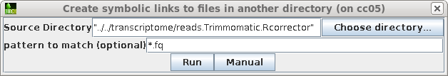
Use the directory chooser to select the name of the directory containing the corrected reads. The chooser will use the fully-qualified path to the files for the symbolic links. The link names can be made shorter by editing the Source Directory line to a relative path ie.
../../transcriptome/reads.Trimmomatic.Rcorrector

In either case, set the pattern to "*.fq" and click on Run.

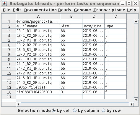
The blreads window will refresh, showing the symbolic links to the read files.

To download gzipped files

Next, download the .fq.gz files found at ftp://ftp.cc.umanitoba.ca/psgendb/BIRCH/data/blreads/de/reads.Trimmomatic.Rcorrector . The files contain the corrected reads, which should be saved to your reads directory. The total size of these files is around 2.3 Gb.

Next unzip the files, using either unpigz (faster) or gunzip:

unpigz *.gz

or

gunzip *.gz

Verify that the files have been unzipped correctly:

ls -l
total 8623152
-rw-rw-r-- 1 psgendb psgendb 654227590 Mar 21 13:27 18-1_R1_val_1.cor.fq
-rw-rw-r-- 1 psgendb psgendb 657474671 Mar 21 13:27 18-1_R2_val_2.cor.fq
-rw-rw-r-- 1 psgendb psgendb 631270036 Mar 21 13:31 18-2_R1_val_1.cor.fq
-rw-rw-r-- 1 psgendb psgendb 630134395 Mar 21 13:31 18-2_R2_val_2.cor.fq
-rw-rw-r-- 1 psgendb psgendb 645589447 Mar 21 13:36 18-3_R1_val_1.cor.fq
-rw-rw-r-- 1 psgendb psgendb 647000420 Mar 21 13:36 18-3_R2_val_2.cor.fq
-rw-rw-r-- 1 psgendb psgendb 632249759 Mar 21 13:40 24-1_R1_val_1.cor.fq
-rw-rw-r-- 1 psgendb psgendb 631184299 Mar 21 13:40 24-1_R2_val_2.cor.fq
-rw-rw-r-- 1 psgendb psgendb 799667084 Mar 21 13:45 24-2_R1_val_1.cor.fq
-rw-rw-r-- 1 psgendb psgendb 798155913 Mar 21 13:45 24-2_R2_val_2.cor.fq
-rw-rw-r-- 1 psgendb psgendb 1035312919 Mar 21 13:51 24-3_R1_val_1.cor.fq
-rw-rw-r-- 1 psgendb psgendb 1033130655 Mar 21 13:51 24-3_R2_val_2.cor.fq

At this point, one way or another, you now have either read files or symbolic links to read files in your de/reads directory.

1. Index the annotated genome using Hisat2-build

To make it more efficient for Hisat2 and Stringtie to work with the annotated genome, we need to build a number of index files to the genome and its features.

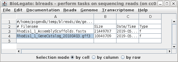
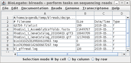
Go to the de/genome directory and launch blreads.

Select the GFF3 file as shown.

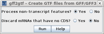
Next, choose Transcriptome --> gff2gtf. This command uses gffread to convert gff or gff3 files into the GTF format needed by Hisat2.

You may wish to set the two parameters which govern which annotations go into the GTF file. In this case choose "Yes" for Process non-transcript features.

The blreads window will be refreshed to show that the GTF file has been created.

Hisat2 requires separate files for annotation of exons and splice sites. Choose Transcriptome --> extract_exons.py and choose the GTF file.

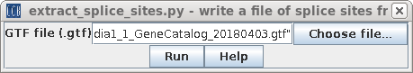
Next, choose Transcriptome --> extract_splice_sites.py and again choose the GTF file.

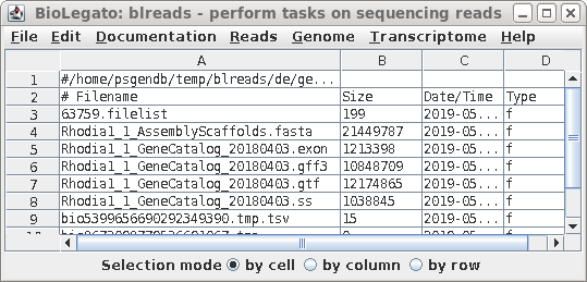
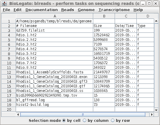
Now, the exon (.exon) and splice site (.ss) files should also be visible in blreads.

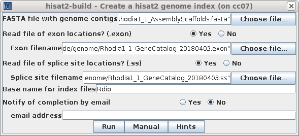
At this point we are ready to create the Hisat index files using hisat2-build.

Choose Transcriptome --> hisat2-build. Select Rhodia1_1_AssemblyScaffolds.fasta, and the exon and splice site files. Remember to click "Yes" to tell blreads to use the exon and splice site files.

Click on Run to start hisat2-build.

A new blreads window will appear showing the creation of eight .ht2 files, which will be used in subsequent steps.

2. Create .bam files, mapping the reads to annotated features in the genome using Hisat2.

The next step is to create .bam files which contain reads mapped to the genome. Because this step utilizes the corrected reads, we need to run blreads in the de/reads.Trimmomatic.Rcorrector directory. Use guesspairs.py to group read pair files, as shown: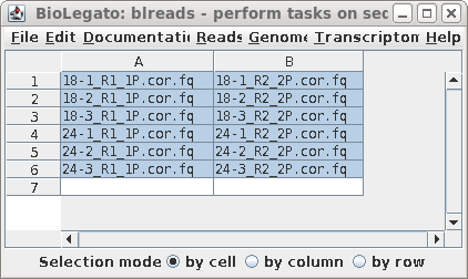

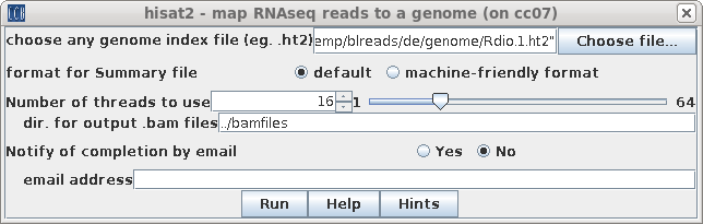
Choose any of the .ht2 files (eg. Rdio_1.ht2).

Output will be written to de/bamfiles, by default.

Click on Run.

For each pair of read files, hisat2 will write a .sam file mapping the read pairs to the genome. Because stringtie will require the reads to be sorted by position in the reference genome, the .sam files are read and sorted by samtools, and output written to .bam files, which contain the same information in smaller binary format. The .sam files are deleted. A new blreads window will open in the bamfiles directory.

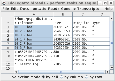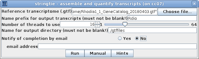
3. Map reads to annotated transcripts using stringtie

Stringtie assembles the reads on to transcripts, mapped to the annotated genome.

First, make sure that the .bam files from the previous step are all selected. Next, choose Transcriptome --> stringtie.

Choose the RTF file created in step 1 as the reference transcriptome.

Type in a prefix which will be part of the name of each transcript written to the output. These names will be used in all downstream analysis, so make it meaningful, but short.

By default, output will be written to a directory called de/gtffiles.

When stringtie is finished, for each .bam file in the bamfiles directory, there is now a GTF file in the gtffiles directory.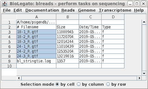

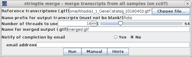
Next, we need to create a merged file containing the information from all of the GTF files. Select all of the GTF files produced in the previous step and choose Transcriptome --> stringtie merge.

Again, we chose the genome GTF file as the reference transcriptome, and set the prefix to "Rdio".

Output will be written to the gtffiles directory to a file called merged.gtf.

It is a good idea to evaluate how well the reads map to the reference transcriptome. Gffcompare generates a number of useful statistics by comparing the merged transcriptome with the annotated transcriptome. In particular, because we are using a small subset of reads with low coverage of the genome, we probably don't want to trust new transcripts that were not annotated in the complete genome. This is especially true because the test dataset for this tutorial was derived from the original dataset used to annotate the genome in the first place.

At this juncture, it is critical to note that the situation might be reversed with real-world data. For example, if the experimental data being used was from a tissue, condition or treatment not represented in the original annotated genome, there could very well be new transcripts that had not been annotated before. In that case, we would want to retain novel transcripts.

For the purposes of this tutorial, we will proceed assuming that we don't want novel transcripts.

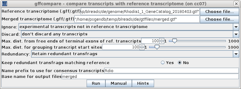
To run gffcompare, choose Transcriptome --> gffcompare.

Again, select the GTF file for the reference genome, and the merged transcriptome file, merged.gtf from the gtffiles directory.

Select Ignore: experimental transcripts not in the reference genome.

Once again, specify "Rdio" as the prefix for transcripts. Click on Run.

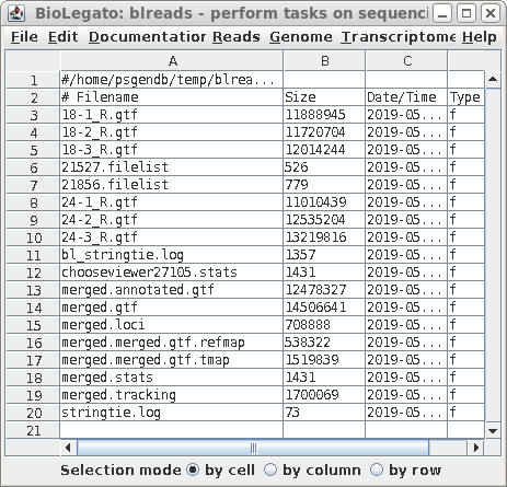
A new blreads window will pop up in the gtffiles directory.

Merged.annotated.gtf contains the transcripts from merged.gtf, minus the novel experimental transcripts.

The file merged.stats contains a report showing both the sensitivity (fraction of true transcripts found) and the precision, true transcripts as a fraction of false positives and true positives.

Keep in mind that the next step generates the actual differential expression data that you will use in all downstream analysis of your experiment. For that reason, it is a good idea to read carefully the Gffcompare manual to understand the results.

In short, we can say that 100% of the loci, bases, exons, and introns from the annotated genome were found in the experimental transcriptome. The 99.9% Precision estimate says that a few novel loci were inferred from the experimental data.

81.1% of the exons found in the experimental data correspond to annotated exons, meaning that 19.9% of the exons are novel exons. When we look at transcripts, only 62.6% of the transcripts from the experiment were also seen in the annotated genome, meaning that 37.4% of the exons are novel, probably artifacts due to the small size of the dataset. (If this was RNAseq data from a new condition not represented in the annotated transcriptome, these novel exons or transcripts might be newly discovered, but legitimate exons, transcripts etc.)

It may be a good idea to re-run gffcompare with different parameters, or go back to try different assembly parameters, before commiting to the final step.

4. Calculate FPKM statistics from mapped reads using stringtie -B

When you are satisfied with a set of merged transcripts, it is time to run stringtie again to generate FPKM and other statistics for use by Ballgown or other downstream gene expression systems.

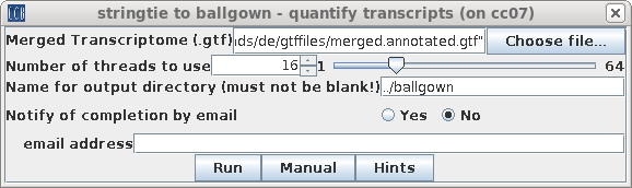
Because we now want to use the reads to measure gene expression levels for the annotated transcripts.

Open blreads in the bamfiles directory, select all .bam files
and choose Transcriptome --> stringtie to ballgown, and set the merged transcriptome file to merged.annotated.gtf.

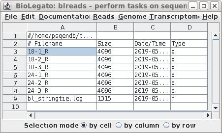
The results will be written to the ballgown directory.

Note that almost all of the contents of the ballgown directory consists of subdirectories, one for each .bam file.

The contents of each subdirectory can be viewed in either a file manager, or in blreads. For example, to view the contents of 18-1_R, choose 18-1_R, and then File --> Open directory.

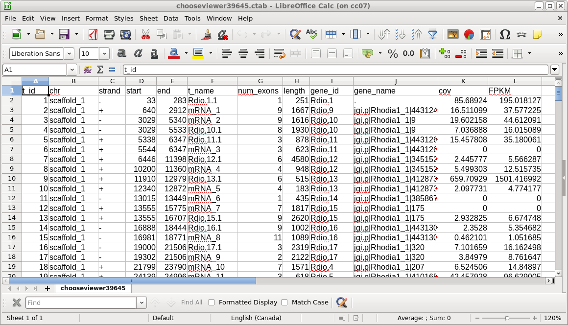
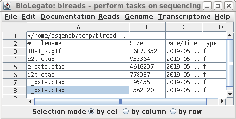
Each directory has a gtf file for one set of reads, as well as a number of CSV files with the .ctab file extension.

The most important one is t_data.ctab, which has the FPKM calculations for each transcript. You can view this file by selecting t_data.ctab, and then File --> View file.

More information on how to use these files with the Ballgown R package can be found at https://github.com/alyssafrazee/ballgown#ballgown-readable-expression-output.

Ballgown is not part of the current BIRCH release, but can be installed separately, from the above site.